Introduction to 3D Plotting using MATLAB plot3
Data visualization is a crucial aspect of data analysis, allowing us to interpret complex datasets and recognize patterns or trends that might otherwise go unnoticed. In the field of data science and engineering, 3D plotting serves a vital role, as it enables a more intuitive representation of multidimensional data. MATLAB, a powerful software tool popular in academia and industry, provides the plot3 function to facilitate the creation of three-dimensional plots with relative ease.
The plot3 function in MATLAB simplifies the graphical representation of three-dimensional data by allowing users to plot points, lines, and surfaces in a Cartesian coordinate system. This functionality caters to a diverse audience, ranging from beginners who are just starting to explore data visualization techniques to experienced programmers looking to enhance their graphical presentations. By enabling a spatial understanding of data, 3D plotting becomes essential in various scenarios such as engineering simulations, scientific research, and statistical analysis.
Common use cases for 3D visualizations using MATLAB include representing geographical data, displaying complex mathematical functions, and illustrating results from experiments or simulations. Visualizing such data in three dimensions can reveal relationships between variables that are not immediately obvious in two-dimensional plots. Additionally, industries such as computer graphics, robotics, and physics frequently leverage 3D visualizations to represent spatial data accurately.
The ability to effectively use the plot3 function can significantly enhance communication of data insights, making it an invaluable tool in a data analyst’s toolkit. As we dive deeper into the specifics of the plot3 function in the following sections, we will explore its syntax, parameters, and practical applications to unlock its full potential in your data visualization pursuits.
Understanding the Basics of plot3
The plot3 function in MATLAB is an essential tool for creating three-dimensional plots. Understanding its syntax and functionalities forms the groundwork for more advanced 3D visualizations. The primary function syntax is plot3(X, Y, Z), where X, Y, and Z are vectors of the same length representing coordinates in a 3D space. Each coordinate is essential for plotting points that make up the 3D line or surface.
The X vector corresponds to the horizontal axis, the Y vector represents the vertical axis, and the Z vector indicates depth. By providing these three sets of data, users can visualize complex datasets in a manner that enhances understanding and interpretation. One of the simplest forms of utilizing the plot3 function involves substituting these vectors with specific numerical values or arrays.
For instance, if one were to plot a simple helix, they could define the vectors as follows:
X = sin(t)
Y = cos(t)
Z = t;
Here, t would be a linearly spaced vector defining the range over which the function is evaluated. The result would yield a 3D spiral, making it easy to comprehend how mathematical functions can manifest visually in three dimensions.
Moreover, the plot3 function allows for additional customization options such as color, markers, and line styles. By specifying optional arguments, users can enhance the readability of their plots. Understanding these essential features equips users with the foundational skills needed to create their first 3D plot in MATLAB and serves as a stepping stone for more sophisticated visualizations.
Additionally, Python offers the capability to create dynamic 3D scatter plots, which can greatly enhance data visualization and interpretation. Moreover, it is noteworthy that Python can be seamlessly integrated and executed within the MATLAB environment, allowing users to leverage the strengths of both programming languages. This integration empowers developers and researchers to harness Python’s libraries and tools while working efficiently within MATLAB. Embracing this approach can significantly broaden your analytical and graphical representation skills, making it essential to learn how to effectively utilize Python within the MATLAB ecosystem.
Customizing Your 3D Plots with MATLAB plot3
Customizing 3D plots in MATLAB using the plot3 function is vital for effective data visualization. Users have multiple options available to enhance the clarity and aesthetic appeal of their plots. To start, changing line styles, colors, and markers can significantly alter the visual impact of a plot. For instance, you can use the following syntax to modify the line style: plot3(x, y, z, 'line_style'). Common line styles include solid, dashed, and dotted lines, which can be represented as ‘-‘, ‘–‘, and ‘:’, respectively. Furthermore, incorporating colors can be achieved by specifying a color in the plot command, such as plot3(x, y, z, 'r--') for a red dashed line.
Markers are another customization feature that helps to distinguish data points within the 3D space. The plot3 function allows users to include various marker styles, such as circles, squares, or diamonds, by appending an appropriate character, like ‘o’, ‘s’, or ‘^’, to the line specification. For example, plot3(x, y, z, 'ro') plots the data points with red circular markers, providing clarity in dense data sets.
Beyond line styles and markers, adding labels, titles, and legends is crucial for clearly conveying information within your 3D plots. Use the xlabel, ylabel, and zlabel functions to define descriptive axes labels, helping viewers understand what each axis represents. Additionally, adding an overall title with the title function enhances the plot’s context. Implementing a legend using the legend function aids in clarifying what different lines represent, especially when multiple datasets are displayed simultaneously. By thoughtfully customizing 3D plots with these features, users can create visually engaging and informative representations of their data using the MATLAB plot3 function.
Adding Grids and Axes to Your Plots using MATLAB plot3
In the realm of 3D visualization, particularly when working with MATLAB’s plot3 function, the inclusion of grid lines and well-defined axes plays a vital role in the interpretation of data. Grids assist the viewer in assessing values and identifying trends, while axes provide crucial reference points that enhance the plot’s clarity. The activation of grid lines in MATLAB is straightforward; simply use the grid on command after your plot3 call. This not only introduces visual cues on the plot surface but also helps in aligning data points to their respective coordinates.
Customizing axis limits is another critical aspect that can significantly improve a plot’s usability. By using commands such as xlim, ylim, and zlim, users can set the ranges for each axis, allowing for focus on specific data regions. This is particularly useful when the data being visualized contains outliers or when specific ranges are of interest. For example, if you want to restrict the x-axis to start from zero and go up to a particular maximum value, you would utilize xlim([0,maxValue]), where maxValue is your desired upper limit.
Furthermore, the formatting of axes in plots created with the plot3 function enhances readability and presentation quality. MATLAB offers options such as xlabel, ylabel, and zlabel to label each axis accurately, providing context to the viewer about what each axis represents. Additionally, employing the title function to add descriptive titles can further contribute to the overall understanding of the plotted data. Combining these features allows for a more meaningful representation where viewers can easily navigate through the 3D plot and extract insights. By adhering to these practices, the effectiveness of MATLAB’s plot3 function is greatly augmented, leading to an improved analytical experience.
Enhancing Interactivity with MATLAB Tools
Interactivity is a critical aspect of visual data representation, particularly when dealing with 3D visualizations such as those produced using the MATLAB plot3 function. With the built-in tools provided by MATLAB, users can easily manipulate their 3D plots, allowing for a more comprehensive examination of the data. Features such as rotation, zooming, and panning enable users to gain different perspectives on the same dataset, enhancing understanding and engagement.
To rotate a 3D plot in MATLAB, users can click and drag within the axes of the plot. This action allows the user to view the data from various angles, a crucial feature when trying to understand complex three-dimensional structures. Similarly, zooming in and out can be achieved using the mouse scroll wheel or by utilizing the zoom tool in the MATLAB figure toolbar. This allows for closer examination of specific areas within the 3D visualization, providing more detail than what might be visible at a broader perspective.
Panning is another essential function that can be performed in MATLAB to move the view without altering the scale of the plot. Employing the pan tool from the MATLAB axes toolbar, users can shift the view around the plot, allowing for a more versatile exploration of the visualized data. This functionality is particularly beneficial when users are interested in targeting specific data regions without losing sight of the overall dataset.
To further enrich interactivity, MATLAB also supports the use of callbacks and custom functions. By linking specific user actions, such as mouse clicks or key presses, to predefined functions, users can create dynamic and responsive 3D visualizations. For example, a callback function could update the data displayed in a plot or modify the viewpoint directly in response to user inputs. This level of interactivity not only improves the visual experience but also fosters deeper engagement with the dataset being analyzed.
Advanced Techniques: Surface and Volume Plots using MATLAB plot3
While MATLAB’s plot3 function excels in rendering basic three-dimensional line plots, it also lays the foundation for more intricate visualizations, such as surface and volume plots. These advanced techniques are essential for effectively showcasing complex datasets, allowing researchers and engineers to glean deeper insights from their data.
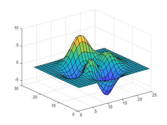
To create a surface plot, users can utilize the surf function, which can be combined with the meshgrid function to generate a grid of values. For instance, consider the following sample code:
[X, Y] = meshgrid(-5:0.5:5, -5:0.5:5)
Z = sin(sqrt(X.^2 + Y.^2))
surf(X, Y, Z);
This snippet generates a surface plot depicting a three-dimensional sine wave pattern. It provides a more comprehensive view of how the Z values change over the X and Y planes.
Volume visualization is another powerful technique that can be employed, often using functions like slice or isosurface. Volume plots are particularly useful in fields such as medicine or fluid dynamics, allowing practitioners to visualize complex volumetric data. Below is an example using the isosurface function:
[X, Y, Z] = meshgrid(-5:0.5:5, -5:0.5:5, -5:0.5:5)
V = X.^2 + Y.^2 + Z.^2
isosurface(X, Y, Z, V, 20)
This code snippet generates an isosurface of the 3D volume defined by the equation, offering a tangible representation of the data. Using plot3 as an underlying tool, users can effectively transition from basic line plots to sophisticated surface and volume renderings, enhancing their data visualization capabilities in MATLAB.
Learn MATLAB with Online Tutorials
Explore our MATLAB Online Tutorial, your ultimate guide to mastering MATLAB! Whether you’re a beginner or an advanced user, this guide covers everything from basic MATLAB concepts to advanced topics
Use Cases in Data Science and Engineering
The matlab plot3 function plays a significant role in the visualization of complex datasets across various fields, particularly in data science and engineering. One primary application is in understanding multivariate data. In many scenarios, engineers and data scientists deal with variables that jointly influence outcomes, and utilizing a three-dimensional visualization through plot3 enables them to better understand correlations and interactions among these variables. For instance, an engineer might use this function to plot the performance metrics of machines against their operational parameters, thereby presenting a clearer picture of how different inputs affect outputs.
Another practical usage of matlab plot3 is in the realm of geospatial analysis. Here, the function can be employed to visualize geographic data, allowing for a deeper understanding of spatial relationships. For example, researchers can plot the results of environmental studies, illustrating how pollution levels vary across different locations. By representing this data in three dimensions, stakeholders can easily identify trends, hotspots, and potential areas of concern.
Furthermore, the plot3 function is essential when analyzing scientific data. In fields such as physics and biology, where numerous variables operate concurrently, 3D plots serve as effective tools to convey findings comprehensively. A clear exemplification is in molecular modeling. Scientists can employ MATLAB’s plot3 to visualize complex molecular structures and their interactions, helping elucidate their behavior in various contexts.
In industries such as automotive and aerospace engineering, matlab plot3 is frequently utilized for analyzing and visualizing complex aerodynamic designs. By plotting airflow patterns and pressure distributions in a three-dimensional space, engineers can optimize designs for better performance, contributing to more efficient vehicles and aircraft.
Overall, the versatility of the matlab plot3 function enables professionals across numerous domains to visualize their findings effectively, facilitating not only analysis but also informed decision-making.
Common Challenges and Troubleshooting Tips
When working with MATLAB’s plot3 function for 3D visualization, users often encounter several challenges that can affect their ability to effectively portray data. One common issue is misunderstanding the axes scaling. In 3D plots, the default scaling may not reflect the actual distribution of data points, leading to misinterpretations. For instance, if one axis extends significantly further than the others, this could distort the visual representation, making it crucial to manage axis limits explicitly using the xlim, ylim, and zlim functions to achieve a coherent view.
Another challenge arises from the data types being used in the plot3 function. It is essential that the data inputs for the x, y, and z coordinates are correctly formatted and of compatible types. Users may inadvertently input incompatible matrix dimensions, which can result in errors. Conducting preliminary checks of the dimensions of the arrays can help mitigate this issue. Additionally, it is advisable to employ built-in functions such as size and length to validate data before invoking the plotting function.
In terms of rendering the plots, performance can decline significantly when handling large datasets, leading to slow responsiveness. To improve visual performance, users can reduce the number of points plotted by subsampling the data. This approach maintains the general shape and trends of the data without overwhelming the rendering engine. Additionally, adjusting rendering settings or simplifying the plot by utilizing fewer graphical elements can enhance the interaction experience.
Users may also experience challenges related to the graphical display itself, such as plots not appearing as expected or disappearing. In such cases, ensuring that the figure window is appropriately configured and that the visibility settings are correct can resolve these issues. By addressing these common pitfalls and following the provided troubleshooting tips, users can significantly improve their proficiency with the plot3 function in MATLAB, leading to more effective and intuitive 3D visualizations.
Conclusion and Future Directions
In this blog post, we have explored the MATLAB plot3 function, which serves as a powerful tool for visualizing 3D data. We discussed its features, capabilities, and potential applications across various fields, emphasizing how this function allows users to plot points, lines, and surfaces in a three-dimensional space effectively. Beginners and experienced users alike can benefit from understanding the nuances of 3D plotting, as it enhances the ability to interpret complex data sets visually.
Throughout our discussion, we highlighted key components of the plot3 function, such as specifying coordinates, customizing plot aesthetics, and utilizing additional functions for improved visual representation. Understanding the syntax and utilities available within the MATLAB environment is crucial to maximizing the efficiency of the plot3 function. We also covered various techniques for elevating your 3D plots, such as adjusting camera angles and lighting, which further enhance data visualization.
As we look to the future, it is essential to stay informed about advancements in data visualization tools and practices. The MATLAB documentation is an invaluable resource for anyone looking to deepen their understanding of plot3 and explore similarly powerful functions. In addition to the basic capabilities we discussed, there are many advanced topics worth investigating, such as surface plots, mesh grids, and interactive visualization techniques that can significantly enrich one’s data analysis repertoire. By continuously exploring these aspects, users can elevate their skills and apply them to more complex data challenges.
By mastering the plot3 function and engaging with the broader suite of MATLAB visualization tools, practitioners will be well-equipped to tackle the demands of modern data analysis, driving deeper insights and promoting informed decision-making.
MATLAB Ode45 function – Practical Tutorials
Ode45 is a widely utilized numerical solver designed for the effective resolution of ordinary differential equations (ODEs). It is a part of MATLAB’s ODE suite and is specifically tailored to handle problems where the solution requires the calculation of derivatives at multiple points. The significance of Ode45 stems from its implementation of the Runge-Kutta method, which offers a robust approach to approximating solutions with high accuracy.
MATLAB Diff function – Beginners Tutorials
MATLAB diff function is an essential tool utilized in the realms of data analysis and programming. Primarily, it calculates the differences between adjacent elements in an array, offering valuable insights into trends and behaviors of data sets. Through a blend of theoretical understanding and hands-on practical examples on MATLAB, this guide aspires to empower readers to utilize MATLAB’s diff effectively, transforming raw data into actionable insights.
MATLAB conv2 Function
Convolution is a mathematical operation that combines two functions to produce a third function, expressing how the shape of one function is modified by the other. Convolution is calculated using MATLAB conv2 function. This operation is particularly crucial in various fields such as image processing, signal analysis, and systems engineering. This function is specifically designed for two-dimensional convolution, making it preferable for tasks that involve images or other matrix-based data
fft2 in MATLAB
The FFT2 function in MATLAB is crucial for performing Fourier transforms on matrices, allowing practitioners to study and manipulate two-dimensional frequency components effectively. The Fast Fourier Transform (FFT) is an algorithm that computes the discrete Fourier transform (DFT) and its inverse efficiently. The DFT converts a sequence of equally spaced samples of a function into a sequence of coefficients of sinusoidal components, revealing the frequency spectrum of the sampled signal.
fzero MATLAB Function
The fzero in MATLAB is a powerful tool designed for finding the roots of nonlinear equations. This function plays a crucial role in various fields, including engineering, data science, and mathematical modeling. By utilizing fzero MATLAB, users can efficiently identify points where a given function equals zero, which is essential for solving problems that involve polynomial equations, differential equations, and optimization tasks.
MATLAB interp1 Function
The interp1 function in MATLAB serves as a fundamental tool for conducting one-dimensional interpolation on a set of data points. Interpolation is a statistical method that estimates values between two known values, allowing for more precise data analysis and management. By employing the interp1 function, users can obtain interpolated values at specified points, thus enabling a deeper analysis of datasets.