Introduction to Linear Regression
Linear regression represents a pivotal method in statistical analysis and data science, enabling researchers and analysts to model relationships between variables. This blog post provides a comprehensive introduction to linear regression and its implementation on MATLAB. At its core, linear regression seeks to establish a linear equation that best describes the relationship between a dependent variable and one or more independent variables. This technique is widely utilized in various fields, including economics, health sciences, social sciences, and machine learning, making it essential for those looking to derive meaningful insights from data.
The primary objective of linear regression is to predict the value of a dependent variable based on the values of independent variables. By fitting a line (or hyperplane in multi-dimensional contexts) to a scatter plot of data points, linear regression provides a straightforward interpretation of how changes in the independent variables affect the dependent variable. This is particularly valuable in scenarios where understanding these relationships can inform decision-making or strategy. For instance, in a business context, one might use linear regression on MATLAB to predict sales based on advertising spend, thereby highlighting the importance of marketing investments.
In MATLAB, linear regression can be efficiently executed using built-in functions that facilitate not just the computation of regression coefficients but also allow for the assessment of the model’s performance through metrics such as R-squared and residual analysis. When performing a linear fit on MATLAB, one can readily visualize the results, enabling an enhanced understanding of the data and the model itself. Furthermore, linear regression forms the foundation for other advanced statistical techniques, including polynomial regression and multi-variable regression analysis, thus underscoring its significance in the broader landscape of statistical modeling.
Overall, mastering linear regression using MATLAB equips professionals with a robust toolkit for data analysis, allowing them to translate complex datasets into actionable insights. Its fundamental nature is what makes understanding linear regression on MATLAB a necessary skill for those involved in data-driven decision-making.

Introduction to MATLAB
MATLAB, short for Matrix Laboratory, is a high-performance programming language and environment primarily used for numerical computing, data analysis, algorithm development, and visualization. It excels in handling matrices, making it a preferred tool for mathematical modeling and analysis. For users interested in performing linear regression on MATLAB, understanding its environment and functionalities is crucial.
Installation and Environment Overview
To begin with MATLAB, users must first download and install the software from the official MathWorks website. The installation process is straightforward: after downloading, run the installer, follow the on-screen instructions, and activate the software using a license. Once installed, opening MATLAB presents users with a user-friendly interface, which consists of several panes. The command window is where users can execute commands directly, while the workspace displays variables created in the session. The command history keeps a log of previous commands, enhancing the workflow.
Basic Functionalities for Data Analysis
MATLAB offers essential commands that facilitate data manipulation and analysis, enabling users to perform a linear fit effortlessly. Users can import datasets using commands like readtable or csvread, which allows for easy access to tabular data. Basic operations such as indexing, sorting, and filtering can be managed using built-in functions. For those focusing on linear regression, incorporating the fitlm function is crucial, as it applies MATLAB’s linear regression features efficiently, providing outputs such as coefficients, statistics, and residuals.
Conclusion
In summary, understanding the basics of MATLAB is vital for users looking to perform linear regression analysis. Familiarity with its interface, installation process, and essential commands provides a strong foundation for utilizing MATLAB’s powerful capabilities in data analysis and linear fitting.
Need Help in Programming?
I provide freelance expertise in data analysis, machine learning, deep learning, LLMs, regression models, NLP, and numerical methods using Python, R Studio, MATLAB, SQL, Tableau, or Power BI. Feel free to contact me for collaboration or assistance!
Follow on Social

Preparing Your Data for Linear Regression
Data preparation is a crucial step before performing linear regression on MATLAB. The quality of your dataset significantly impacts the accuracy of your model, making it essential to follow systematic techniques for data cleaning, processing, and visualization.
The first step in preparing your data involves cleaning. This means identifying and handling any missing values within your dataset. In MATLAB, you can use functions such as isnan to detect missing entries. Once identified, you can opt to either remove these rows or impute values based on the overall trends within your data. It is also important to check for outliers using visualization techniques like box plots or scatter plots. Outliers can skew your linear regression results, so addressing them should be of utmost priority, either through removal or correction.
Subsequently, processing your data becomes necessary to ensure it is in a suitable format for analysis. This includes standardizing or normalizing numerical variables, which can improve the performance of your model by ensuring all input features have similar scales. MATLAB offers normalization functions that can streamline this process, allowing for efficient manipulation of your data entries.
Visualization plays a vital role in understanding the relationships within your data. Prior to fitting a linear model, use MATLAB’s plotting capabilities to create scatter plots for the pair of independent and dependent variables. This visual inspection helps to assess whether a linear relationship exists between the variables and informs the decision for applying a linear regression model to your dataset.
Finally, loading datasets into MATLAB is straightforward. Through commands such as readtable or load, you can easily import data from various file formats, ensuring that your data is ready for analysis. By following these preparatory steps for linear regression in MATLAB, you lay a strong foundation for accurate modeling and reliable results.
Implementing Linear Regression in MATLAB Code
To implement linear regression in MATLAB, one can utilize built-in functions that streamline the process of fitting a linear model to data. The most common approach is to use the ‘fitlm’ function, which allows users to specify predictor and response variables conveniently. For instance, given a dataset with independent variables represented in matrix form and a dependent variable as a vector, executing the command mdl = fitlm(X, Y) will generate a linear regression model where X contains the predictors and Y the response data.
Once the model is created, it is crucial to interpret the outputs effectively. The coefficients extracted from the model output indicate the relationship between each predictor and the dependent variable. Each coefficient quantifies how much the dependent variable is expected to increase when the respective predictor increases by one unit, holding other predictors constant. The intercept, which is also part of the output, represents the expected value of the response variable when all predictor variables are zero.
Goodness-of-fit measures are essential for understanding how well the model fits the data. Metrics such as R-squared and Adjusted R-squared are typically provided in the output. R-squared reflects the proportion of the variance in the dependent variable that can be explained by the model. A higher R-squared value indicates a better fit. In contrast, Adjusted R-squared accounts for the number of predictors in the model, thus preventing overfitting, which is crucial when conducting linear regression on MATLAB.
Tuning the model may also include checking residuals to assess linearity assumptions and refining the selection of predictors based on statistical significance and practical relevance. By leveraging these steps with MATLAB’s powerful linear regression capabilities, one develops a robust understanding of modeling relationships in data efficiently.
% Linear Regression in MATLAB
% Generate synthetic data
x = linspace(0, 10, 100)'; % Feature values
y = 3 * x + 7 + randn(size(x)); % Linear relation with noise
% Add a column of ones to x for the intercept term
X = [ones(size(x)), x];
% Compute parameters using the Normal Equation
theta = (X' * X) \ (X' * y);
% Predicted values
y_pred = X * theta;
% Plot the data and regression line
figure;
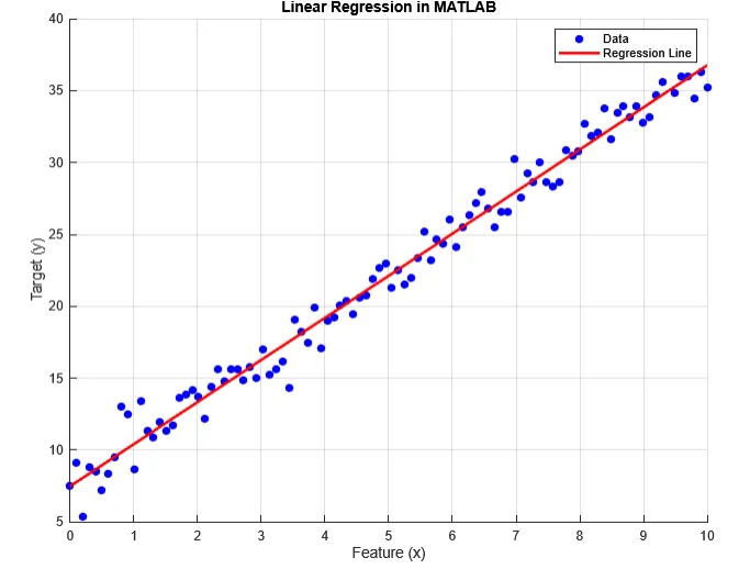
scatter(x, y, 'b', 'filled'); % Scatter plot of data
hold on;
plot(x, y_pred, 'r', 'LineWidth', 2); % Regression line
xlabel('Feature (x)');
ylabel('Target (y)');
title('Linear Regression in MATLAB');
legend('Data', 'Regression Line');
grid on;
hold off;
% Display computed coefficients
disp('Computed coefficients (theta):');
disp(theta);
Output:
Computed coefficients (theta):
7.4736
2.9299
Evaluating Model Performance
Evaluating the performance of a linear regression model is crucial to ensure that its predictions are accurate and reliable. Several metrics and techniques can be employed to assess this performance effectively when using linear regression in MATLAB.
One of the primary metrics used is the R-squared value, which indicates the proportion of variance in the dependent variable that can be explained by the independent variables in the model. In MATLAB, this can be easily calculated using built-in functions after fitting a model. A higher R-squared value signifies that the model explains a significant amount of the variability in the outcome data, thus suggesting a better fit. However, it is essential to interpret this metric cautiously, as a high R-squared does not always equate to a meaningful relationship.
In addition to R-squared, residual analysis is another vital step in evaluating the model’s performance. Residuals, the differences between observed and predicted values, should ideally be randomly distributed with no discernible patterns. In MATLAB, residual analysis can be visually examined through scatter plots and histograms. By checking for normality and independence, one can determine whether the linear regression on MATLAB has adequately captured the underlying relationship of the data.
Cross-validation techniques are valuable for assessing how the findings from the model will generalize to an independent dataset. Methods such as k-fold cross-validation allow one to split the dataset into subsets, iteratively using them to train and validate the model. This process not only helps in minimizing overfitting but also provides more reliable estimates of model performance. Implementing MATLAB linear fit functions can facilitate this process, making it easier to evaluate how the linear regression model performs under different scenarios.
Analyzing these metrics and techniques ultimately ensures a comprehensive understanding of the linear regression model’s accuracy and reliability, which is vital for making data-driven decisions.
MATLAB Assignment Help
If you’re looking for MATLAB assignment help, you’re in the right place! I offer expert assistance with MATLAB homework help, covering everything from basic coding to complex simulations. Whether you need help with a MATLAB assignment, debugging code, or tackling advanced MATLAB assignments, I’ve got you covered.
Why Trust Me?
- Proven Track Record: Thousands of satisfied students have trusted me with their MATLAB projects.
- Experienced Tutor: Taught MATLAB programming to over 1,000 university students worldwide, spanning bachelor’s, master’s, and PhD levels through personalized sessions and academic support
- 100% Confidentiality: Your information is safe with us.
- Money-Back Guarantee: If you’re not satisfied, we offer a full refund
Advanced Techniques in Linear Regression
Linear regression is a fundamental statistical method used in modeling the relationship between a dependent variable and one or more independent variables. While basic linear regression is effective, advanced techniques like multiple regression, regularization, and polynomial regression provide enhanced capabilities for more complex datasets.
Multiple regression extends the linear regression model to include multiple independent variables, allowing for a comprehensive analysis of how various factors influence a dependent variable simultaneously. This technique is particularly useful in scenarios where interactions between variables may provide significant insights. Using MATLAB, implementing multiple regression can be accomplished with the built-in functions like fitlm, which streamlines the process of estimating coefficients and assessing model performance.
Regularization techniques, such as Ridge and Lasso regression, are indispensable when dealing with high-dimensional data where the risk of overfitting is pronounced. Ridge regression adds a penalty equivalent to the square of the magnitude of coefficients, effectively shrinking them to prevent overfitting while maintaining all variables in the model. This can be easily executed in MATLAB using the function ridge. On the other hand, Lasso regression penalizes the absolute size of the coefficients, thereby enabling variable selection by forcing some coefficients to zero, which enhances model interpretability. Lasso can be implemented in MATLAB using the lasso function, providing an essential tool for practitioners looking to optimize their linear regression models.
Lastly, polynomial regression allows for modeling non-linear relationships by introducing polynomial terms of predictors. This technique expands the linear regression framework and can be particularly useful when the relationship between variables is more complex than a straight line. In MATLAB, polynomial regression can be achieved through the polyfit function, which fit various polynomial models depending on the degree specified.
Each of these advanced techniques significantly enhances the capabilities of linear regression in MATLAB, allowing for more accurate modeling and better insights from data analysis. By carefully selecting the appropriate method based on the dataset characteristics, practitioners can effectively harness the full potential of linear regression on MATLAB.
Learn MATLAB with Free Online Tutorials
Explore our MATLAB Online Tutorial, your ultimate guide to mastering MATLAB! his guide caters to both beginners and advanced users, covering everything from fundamental MATLAB concepts to more advanced topics.

Visualization of Linear Regression Results
Visualizing the results of linear regression is critical for interpreting and communicating findings effectively. MATLAB offers a robust set of plotting functions that make it easy to create informative visualizations. The first step in this process is to generate a scatter plot of the data points, which allows you to observe the relationship between the independent and dependent variables. To create a scatter plot in MATLAB, the scatter function can be employed, specifying the independent variable on the x-axis and the dependent variable on the y-axis.
Once the scatter plot is in place, adding the linear regression line is essential to illustrate the overall trend in the data. MATLAB’s polyfit and polyval functions can be utilized to compute and plot this line. By fitting a linear model to the data using polyfit, you can obtain the slope and intercept needed to evaluate the regression line. The plot function can then be employed to overlay this line on the scatter plot, enabling a visual representation of the linear fit.
Another important aspect of linear regression analysis is the evaluation of residuals. Creating a residual plot can help diagnose the fit of the model. A residual plot is generated by calculating the difference between observed and predicted values. By plotting the residuals against the predicted values using the scatter function, you can visually assess whether there are patterns that suggest a poor fit. Ideally, the residuals should be randomly scattered around zero, indicating that the linear regression model is appropriate for the data.
In summary, effective visualization of linear regression results in MATLAB is achieved through scatter plots, overlaying regression lines, and examining residuals. These methods collectively enhance the understanding of the model’s performance and the underlying relationships within the data.
Common Challenges and Solutions
When utilizing linear regression on MATLAB, practitioners frequently encounter several challenges that can impact the validity of their models. Understanding these issues is critical for achieving an accurate linear fit. Among the most common challenges are multicollinearity, heteroscedasticity, and model overfitting.
Multicollinearity arises when two or more independent variables in a regression model are highly correlated. This situation can lead to inflated standard errors, making it difficult to discern the individual impact of each variable. One effective solution is to assess the correlation matrix using MATLAB functions like corrcoef to identify closely related predictors. Based on this analysis, one can eliminate redundant variables or apply techniques such as Principal Component Analysis (PCA) to retain the essential information while reducing dimensionality.
Heteroscedasticity refers to the presence of non-constant variance of the error terms across different levels of the independent variable. This situation can violate one of the key assumptions of linear regression, leading to biased estimates and misleading conclusions. A common approach to detect heteroscedasticity in MATLAB is the Breusch-Pagan test, which evaluates whether the variance of the residuals changes with the fitted values. If detected, transforming the dependent variable (for example, applying a logarithmic transformation) can often stabilize variance.
Lastly, model overfitting is a considerable risk when dealing with more complex datasets. It occurs when the model performs exceedingly well on the training data but poorly on unseen data. To combat overfitting, one can use MATLAB’s regularization techniques, such as LASSO or Ridge regression, which introduce penalties for larger coefficients. Cross-validation is also advised to ensure that the model generalizes well to new data, balancing fit and complexity effectively.
By being aware of these common challenges in linear regression on MATLAB and applying the suggested solutions, practitioners can enhance the reliability of their analyses and insights derived from the data.
Real-World Applications of Linear Regression
Linear regression is a fundamental statistical technique that finds extensive applications in various industries, showcasing its versatility and practicality. In finance, for instance, linear regression is employed to model relationships among financial variables, aiding analysts in predicting stock prices, assessing risk, and establishing trends. By utilizing linear regression on MATLAB, financial analysts can develop accurate models that consider multiple factors, such as interest rates and economic indicators, enabling them to make informed investment decisions.
In the healthcare sector, linear regression plays a pivotal role in analyzing patient data. Medical researchers use MATLAB linear fit to correlate symptoms, treatments, and outcomes, thus enhancing the understanding of diseases and treatments. For example, by examining the relationship between dosage levels and patient recovery rates, healthcare practitioners can optimize treatment plans, ultimately improving patient care. Furthermore, predicting patient readmission rates can enable hospitals to allocate resources more efficiently.
Marketing professionals also rely on linear regression to evaluate the effectiveness of advertising campaigns. By analyzing consumer behavior data through linear regression MATLAB functions, marketers can discern how different marketing strategies impact sales. This data-driven approach allows for precise targeting, maximizing return on investment. Additionally, organizations leverage linear regression to segment customers based on purchasing patterns, which aids in developing tailored marketing strategies aimed at enhancing customer engagement and loyalty.
Beyond these examples, linear regression can be applied in numerous fields, including agriculture, real estate, and education. Each of these sectors benefits from data-driven decisions facilitated by the powerful capabilities of linear regression in MATLAB. By understanding and mastering these applications, individuals can effectively harness linear regression techniques in their own projects, improving outcomes and insights.