MATLAB conv2 Function: Convolution in Two Dimensions

Convolution and MATLAB using conv2 Function

Convolution is a mathematical operation that combines two functions to produce a third function, expressing how the shape of one function is modified by the other. Convolution is calculated using MATLAB conv2 function. This operation is particularly crucial in various fields such as image processing, signal analysis, and systems engineering. In the context of signals and systems, convolution is used to analyze the output of a linear time-invariant system when an input signal is applied. Moreover, convolution enables the implementation of filters in image processing, allowing for blurring, sharpening, and edge detection, among other effects.

In practice, convolution in two dimensions is commonly associated with the manipulation of images, where matrices represent pixel values. Each element in the output image is produced by applying a convolution kernel (or filter) to the corresponding neighborhood of input pixels, making this technique invaluable for enhancing image features or reducing noise. With its wide-ranging applications, understanding convolution is essential for practitioners and researchers working with multidimensional data.

MATLAB, a high-level programming language and interactive environment, provides robust and efficient tools for performing convolution operations through its built-in functions, one of which is conv2. This function is specifically designed for two-dimensional convolution, making it preferable for tasks that involve images or other matrix-based data. With powerful computational capabilities and user-friendly syntax, MATLAB simplifies the implementation of convolution, enabling users to focus on algorithm design rather than low-level programming details.

To effectively utilize the conv2 function and understand convolution’s broader implications, familiarity with basic linear algebra concepts and matrix operations is essential. Users should also have a foundational grasp of how convolution operates in different contexts, which will enhance their ability to implement and analyze results accurately in practical applications.

What is MATLAB conv2?

MATLAB’s conv2 function computes the two-dimensional convolution of two matrices. It is commonly used in:

• Image processing (e.g., blurring, sharpening, edge detection)
• Signal processing (e.g., smoothing and filtering 2D signals)
• Numerical computing (e.g., applying kernel-based transformations)

Syntax of conv2

C = conv2(A, B)
C = conv2(A, B, shape)

Where:

• A is the input matrix (e.g., an image or a 2D signal).
• B is the kernel (filter) matrix.
• shape (optional) specifies the size of the output. It can be:
  • 'full' (default) – returns the full convolution.
  • 'same' – returns output the same size as A.
  • 'valid' – returns only the region where B fully overlaps A.

Understanding the MATLAB conv2 Function

The conv2 function in MATLAB is a powerful tool used for performing two-dimensional convolution. This mathematical operation is essential in various fields including image processing, signal processing, and control systems. Convolution is the process where two matrices, or functions, are combined to produce a third matrix, emphasizing how the shape of one affects the shape of another. The conv2 function simplifies this complex operation by providing a straightforward syntax and diverse application options.

The syntax of conv2 is designed to be intuitive. It is typically called in the form of conv2(A, B), where A and B are the input matrices. The first matrix, A, is the data set, while the second matrix, B, is the convolution kernel or filter. The operation involves convolving the array A with the kernel B, resulting in an output that retains the dimensions of A while being modified by B.

When utilizing the conv2 function, one can specify various parameters to control the boundaries of the convolution and the size of the output. Options include specifying the method of convolution such as ‘full’, ‘same’, or ‘valid’. The ‘full’ option returns the full convolution result, while ‘same’ ensures that the output matrix matches the size of A. Conversely, ‘valid’ yields only the output points that are valid given the dimensions of both the input and filter matrices.

Input requirements are critical for successful execution; both matrices must be numerical and can be of any size. The output is also numerical, reflecting the convolution results, which can then be utilized for further analysis or visualization in various applications, demonstrating the versatility of MATLAB’s conv2 function.

Setting Up Your Environment

To utilize the MATLAB conv2 function effectively, it is essential to first set up your environment adequately. The initial step is to install MATLAB, which can be obtained from the official MathWorks website. Choose the version that suits your requirements, keeping in mind that later versions often include enhancements and bug fixes for functions, including conv2.

Once you have downloaded MATLAB, proceed with the installation process. This typically involves following on-screen instructions, where you will have the option to customize your installation by selecting specific toolboxes. For convolution operations, make sure that you have the Image Processing Toolbox installed, as it provides additional functionalities that may extend the capabilities of the conv2 function.

After successful installation, launch MATLAB and configure your environment. This includes setting the working directory where your scripts and data files will reside. Using the Current Folder browser within MATLAB, navigate to the appropriate directory or create a new one to facilitate organized file management. Consider also setting up shortcuts for frequently accessed folders.

Furthermore, ensure that all path settings are correctly configured to include necessary folder directories. This can be done by using the addpath command to include third-party libraries or functions that may enhance the usage of the conv2 function. If your project requires data files, check that they are in the supported formats such as matrices or images, as required by MATLAB.

Lastly, running a quick test script can be helpful in verifying that the conv2 function and all necessary components are functioning correctly. A simple convolution operation using two matrices will validate your setup and ensure that your MATLAB environment is ready for further exploration of multidimensional convolution.

Basic Examples of Using conv2 MATLAB function

The matlab conv2 function is highly useful for performing convolution operations on two-dimensional data. Convolution, in essence, is a mathematical operation used for signal processing and image filtering, which combines two arrays to produce a third array. To illustrate the usage of conv2, we will explore several basic examples featuring simple 2D arrays, also known as matrices.

Let’s start with a straightforward example. Consider two matrices: a small image represented as a matrix, and a kernel that will be used for convolution. For instance, we can define a 3×3 matrix representing an image and a 2×2 matrix as our kernel:

image = [1 2 1;0 1 0;2 1 0]
kernel = [1 0;0 -1];

To apply the convolution using matlab conv2, simply use the following command:

result = conv2(image, kernel, 'same');

The option ‘same’ ensures that the output of conv2 has the same dimensions as the input image. The resulting matrix will reflect the convolution operation, where each pixel’s value is influenced by its neighboring pixels according to the kernel.

Another example can involve a larger kernel, for instance, a 5×5 Gaussian filter, which can be used for smoothing an image:

gaussian_filter = fspecial('gaussian', [5 5], 1)
smoothed_image = conv2(image, gaussian_filter, 'same');

In this scenario, conv2 applies the Gaussian kernel to blur the input matrix, resulting in a softened image. These examples illustrate the basic functionality of the conv2 function, providing a foundation for more complex applications in image processing and analysis.

1. Setting Up Your MATLAB Environment

Before using conv2, ensure you have MATLAB installed. If you’re working with images, consider using the Image Processing Toolbox.

2. Understanding the Basics of Convolution

Convolution works by sliding a filter (kernel) over an input matrix and computing the weighted sum of overlapping elements.

Example: Consider the following input matrix A and kernel B:

A = [1 2 3; 4 5 6; 7 8 9]; % Input matrix
B = [0 -1 0; -1 4 -1; 0 -1 0]; % Example kernel (Laplacian filter)
C = conv2(A, B, 'same'); % Apply convolution
disp(C); % Display the result

3. Exploring Different Convolution Shapes

Each shape affects the output dimensions:

C_full = conv2(A, B, 'full');  % Returns the complete convolution
C_same = conv2(A, B, 'same');  % Keeps output the same size as A
C_valid = conv2(A, B, 'valid'); % Returns only fully overlapped regions

disp('Full Convolution:'), disp(C_full);
disp('Same Convolution:'), disp(C_same);
disp('Valid Convolution:'), disp(C_valid);

4. Applying conv2 for Image Processing

conv2 is extensively used in image processing to apply filters like blurring, sharpening, and edge detection.

Blurring an Image

img = imread('example.jpg'); % Load an image
gray_img = rgb2gray(img); % Convert to grayscale
blur_kernel = ones(5,5) / 25; % Averaging filter
blurred_img = conv2(double(gray_img), blur_kernel, 'same');

imshow(uint8(blurred_img)); % Display the blurred image

Edge Detection Using conv2

edge_filter = [-1 -1 -1; -1 8 -1; -1 -1 -1]; % Edge detection filter
edge_detected = conv2(double(gray_img), edge_filter, 'same');

imshow(uint8(edge_detected)); % Show edges

Adaptive Image Filtering

function apply_filter(image_path, filter_type)
    img = imread(image_path);
    gray_img = rgb2gray(img);

    switch filter_type
        case 'blur'
            kernel = ones(5,5) / 25;
        case 'sharpen'
            kernel = [0 -1 0; -1 5 -1; 0 -1 0];
        case 'edge'
            kernel = [-1 -1 -1; -1 8 -1; -1 -1 -1];
        otherwise
            error('Invalid filter type');
    end

    filtered_img = conv2(double(gray_img), kernel, 'same');
    imshow(uint8(filtered_img));
end

% Example usage:
apply_filter('example.jpg', 'edge');

Smooth Data with Convolution using MATLAB Conv2

% Load and convert image to grayscale
img = imread('example.jpg');
gray_img = rgb2gray(img);

% Define a Gaussian smoothing kernel
gaussianKernel = fspecial('gaussian', [5 5], 1);

% Apply convolution using conv2
smoothed_img = conv2(double(gray_img), gaussianKernel, 'same');

% Display original and smoothed images
figure;
subplot(1,2,1);
imshow(gray_img);
title('Original Image');

subplot(1,2,2);
imshow(uint8(smoothed_img));
title('Smoothed Image with Gaussian Filter');

For large matrices, conv2 provides a faster alternative to imfilter

% Generate synthetic 2D data (e.g., terrain, heatmap)
data = rand(100, 100) * 10; % Random matrix

smoothKernel = ones(5, 5) / 25; % 5x5 average filter

smoothed_data = conv2(data, smoothKernel, 'same');

figure;
subplot(1,2,1);
imagesc(data); colormap(jet); colorbar;
title('Original Data');

subplot(1,2,2);
imagesc(smoothed_data); colormap(jet); colorbar;
title('Smoothed Data with 2D Convolution');

Advanced Usage: Parameters and Options

The MATLAB `conv2` function is a powerful tool for performing two-dimensional convolution, and its versatility is further amplified by several advanced options and parameters. A key aspect of utilizing the `conv2` function effectively lies in understanding how these parameters can be tailored to specific applications. The function supports different boundary options, which determine how the convolution process handles the edges of the input matrices.

When invoking the `conv2` function, users can specify boundary options such as ‘same’, ‘full’, or ‘valid’. The ‘full’ option computes the complete convolution, producing the largest output matrix, whereas ‘same’ returns an output that is the same size as the input. The ‘valid’ option, on the other hand, only returns the valid part of the convolution, hence resulting in a smaller output matrix. How convolution is applied at the edges greatly influences the output, especially in applications such as image processing where edge effects may distort the resulting image.

Additionally, specific parameters within `conv2` allow users to control the convolution calculation directly. For instance, the way to handle multiplication can be adjusted through different data types, affecting both the precision and the performance of the operation. Employing double precision can enhance the accuracy of the results, while single precision might be preferable for performance optimization in less sensitive applications. Furthermore, MATLAB offers options to compute convolution without padding, which conserves memory and processing time in scenarios where only output size matters.

In conclusion, grasping the various parameters and options associated with the MATLAB `conv2` function can significantly improve the efficiency and results of two-dimensional convolution operations. By selecting the appropriate boundary options and managing the convolution process parameters, users can tailor the function to meet their specific needs across diverse applications. Understanding these intricacies forms the backbone of proficient MATLAB usage in complex analytical tasks.

Learn MATLAB with Online Tutorials

Explore our MATLAB Online Tutorial, your ultimate guide to mastering MATLAB! Whether you’re a beginner or an advanced user, this guide covers everything from basic MATLAB concepts to advanced topics

Practical Applications of MATLAB conv2 in Image Processing

The matlab conv2 function serves as an essential tool for various image processing tasks, particularly concerning convolution operations applied in two dimensions. This function enables the manipulation of images through the application of different convolution kernels (filters), which can be used for a range of purposes including edge detection, image blurring, and sharpening. Understanding these applications is crucial for effective image analysis and enhancement.

One primary MATLAB’s application of conv2 is edge detection, which is vital for identifying boundaries within an image. By employing convolution kernels such as the Sobel or Prewitt operators, users can highlight changes in pixel intensity, allowing for the clear delineation of edges. This technique is extensively used in computer vision applications, such as object recognition and image segmentation, where distinguishing boundaries is critical for further analysis.

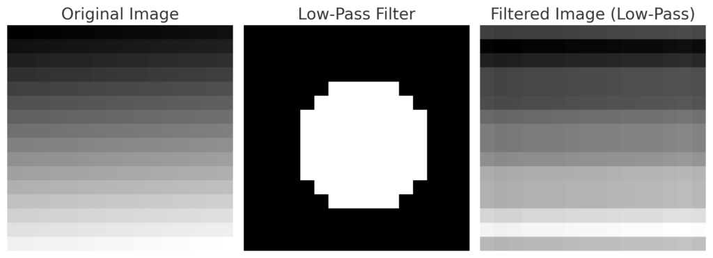
Another significant use of the matlab conv2 function is image blurring. This process is typically achieved through convolution with a Gaussian kernel. The result softens images by averaging pixel values, which effectively reduces noise and facilitates subsequent processing steps. Blurring can be particularly beneficial when preparing images for tasks such as feature extraction, as it aids in minimizing the impact of small, irrelevant details that may otherwise complicate analysis.

Conversely, sharpening is another crucial application enabled by the conv2 function. By utilizing kernels designed to enhance edges, such as the Laplacian filter, the clarity and distinction of features within an image can be markedly improved. This method is common in various fields, from medical imaging to photography, where maintaining detail and sharpness is essential.

In summary, the matlab conv2 function is a potent resource in image processing, allowing for effective manipulation and enhancement through edge detection, blurring, and sharpening. Understanding its applications can significantly influence the quality and usability of image data in various practical scenarios.

Error Handling and Troubleshooting

When using the matlab conv2 function, users may encounter several common errors that can disrupt their workflow. Understanding these potential issues is crucial for effective troubleshooting. One of the most frequent errors is the dimension mismatch between the matrices involved in the convolution. The conv2 function expects inputs to be of compatible sizes. Users should verify that the matrices they are attempting to convolve align in either their rows or columns, as incompatible dimensions will result in runtime errors. To avoid this, it is advisable to check the size of both matrices using the size function prior to invoking the convolution.

Another common issue arises from the presence of NaN values within the matrices. Utilizing matrices containing NaN values with matlab conv2 can lead to unexpected output. Users must ensure that their matrices are clean by conducting data cleansing, potentially utilizing the isnan function to identify non-numeric elements. Filling or removing NaN values beforehand can prevent disruptions in the convolution process.

In addition to these issues, users may experience unexpected results stemming from the choice of the convolution type. Matlab conv2 supports different boundary options such as ‘full’, ‘same’, and ‘valid’. Understanding the implications of each option is essential for attaining the desired output. The ‘full’ option produces an output larger than either input, while ‘same’ aims to produce an output of the same size as the first input matrix, which can lead to confusion if users are not aware of these distinctions. Documentation and MATLAB examples available in MATLAB’s official resources can provide valuable insights when selecting these options.

To summarize, proper understanding of the conv2 function, regular matrix checks, and adherence to MATLAB’s guidelines can significantly ease troubleshooting. Users should familiarize themselves with these common challenges to maintain smooth and efficient workflows.

Performance Optimization Techniques

When utilizing the MATLAB conv2 function, it is essential to consider various performance optimization techniques to enhance efficiency and execution speed. One of the primary factors affecting performance in MATLAB is memory management. High-resolution images or large matrices can lead to increased memory usage, which subsequently slows down processing times. To mitigate this, users should ensure that they are using appropriate data types. For instance, using single precision instead of double precision when possible can significantly reduce memory consumption.

Efficient coding practices also play a crucial role in optimizing the use of conv2. Avoiding unnecessary variable assignments and preallocating matrices can lead to marked improvements in speed. For example, instead of dynamically resizing a matrix within a loop, preallocate the required size before the loop begins. This reduces the overhead caused by MATLAB’s memory reallocation during execution.

Leveraging MATLAB’s built-in functionalities can further enhance the performance of the conv2 function. Functions such as fft2 for performing a Fast Fourier Transform can be especially beneficial. By transforming the input matrices to the frequency domain, convolution can be achieved more rapidly compared to direct spatial convolution. Furthermore, utilizing the parallel computing toolbox allows the distribution of computations across multiple cores, significantly improving processing times for large datasets.

Another best practice is to consider using convolution kernels that are pre-filtered or optimized for your specific needs, as this can steer clear of excessive computation. Employing techniques such as the size of the kernel and input matrix is essential; larger matrices with smaller kernels often lead to better performance. Thus, by understanding these techniques and implementing them thoughtfully, the use of MATLAB’s conv2 can be optimized for enhanced performance, ensuring faster and more efficient computations.

Conclusion and Further Resources

In this comprehensive guide, we have explored the MATLAB conv2 function and its role in performing convolution in two dimensions. The importance of convolution in various applications such as image processing and numerical analysis cannot be overstated. We began by discussing the fundamental concept of convolution and how the conv2 function operates to achieve this mathematical operation. The article provided detailed examples to illustrate the use of conv2, ensuring a clear understanding of how to implement it within different contexts.

Additionally, we highlighted the advantages of using conv2 in MATLAB, such as its efficiency and adaptability when dealing with various matrix sizes and convolution kernels. By comparing the conv2 function to other methods of convolution, we demonstrated its superiority in handling complex data sets and producing high-quality results. Moreover, we examined common pitfalls when using conv2 and offered solutions to enhance its application.

For those looking to further their knowledge on this topic, numerous resources are available. The official MATLAB documentation provides in-depth explanations and additional examples that cater to both beginners and advanced users. Online tutorials, forums, and video courses also serve as excellent supplements for hands-on practice and visual learning. Engaging with these materials will deepen your understanding of the conv2 function and convolution techniques, enabling you to apply them effectively in your projects.

As you continue your exploration of MATLAB’s capabilities, remember that mastering the conv2 function is a pivotal step in leveraging convolution for more advanced data processing tasks. By integrating this knowledge with additional resources, you will enhance your proficiency and apply these powerful computational techniques with confidence.