fft2 in MATLAB

Introduction to fft2 in MATLAB

The Fast Fourier Transform (FFT) is an algorithm that computes the discrete Fourier transform (DFT) and its inverse efficiently. The DFT converts a sequence of equally spaced samples of a function into a sequence of coefficients of sinusoidal components, revealing the frequency spectrum of the sampled signal. In its two-dimensional variant, known as FFT2, this process is extended to analyze digital images and other two-dimensional data sets. The FFT2 function in MATLAB is crucial for performing Fourier transforms on matrices, allowing practitioners to study and manipulate two-dimensional frequency components effectively.

FFT2 proves to be particularly significant in various fields including image processing, signal analysis, and data science. In image processing, for instance, it assists in filtering and enhancing images, revealing features that may not be apparent in the spatial domain. Applications span from medical imaging to remote sensing, where analyzing two-dimensional data sets is essential. Using FFT2 facilitates faster computations than the direct approach of calculating the DFT, significantly improving performance while reducing processing time. For data scientists and programmers, mastering this function allows for more efficient handling and analysis of large datasets.

One of the primary advantages of using FFT2 in MATLAB is its straightforward implementation. The MATLAB environment provides a powerful tool for numeric computation and visualization, enabling rapid prototyping, testing, and debugging of algorithms. By leveraging this built-in function, users can perform complex computations easily, focusing more on the analysis rather than the computational intricacies. Understanding when and how to use FFT2 is crucial; it is particularly useful when dealing with periodic signals or when patterns in data are analyzed. This allows one to transform the data into the frequency domain, facilitating a wide range of analyses.

Understanding the Basics of Fourier Transforms

The Fourier transform is a pivotal mathematical tool extensively utilized in various fields such as engineering, physics, and data science. It provides a powerful method for analyzing the frequency components of signals. Essentially, the Fourier transform decomposes a time-domain signal into its constituent frequencies, allowing researchers and practitioners to study the signal’s behavior in the frequency domain.

At its core, the Fourier transform operates under the premise that any signal can be represented as a sum of sinusoids, each characterized by a specific frequency, amplitude, and phase. This decomposition is pivotal for understanding the underlying structures within the data, as it reveals how different frequency components contribute to the overall shape and characteristics of the signal. The mathematical formulation of the Fourier transform can be expressed as an integral that transforms a continuous function of time into a continuous function of frequency.

For discrete signals, the Discrete Fourier Transform (DFT) is used, which operates on a finite number of samples and processes the signal in a similar manner. The Fast Fourier Transform (FFT) algorithm serves as an efficient computational method for calculating the DFT, significantly reducing the time complexity involved in performing this analysis. Understanding these transformations enables data scientists and programmers to harness the power of frequency analysis, which can be applied in various settings, from signal processing to image analysis.

As we transition into exploring the two-dimensional Fourier transforms, it is crucial to grasp these foundational concepts. Mastery of the one-dimensional Fourier transform will enhance our capability to analyze and interpret more complex signals and images, setting the stage for advanced applications in data science and programming.

Applying FFT2: Practical Applications and Use Cases

The Fast Fourier Transform (FFT) algorithm, particularly its two-dimensional variant, FFT2, has become essential in various fields due to its efficiency in computations involving frequency analysis. One of the most significant applications of FFT2 is in the realm of image processing. Images can be represented as 2D matrices, allowing FFT2 to decompose an image into its frequency components. This transformation is invaluable for tasks such as image filtering, where certain frequencies may need to be suppressed or enhanced to improve image clarity or remove noise. For example, in medical imaging, FFT2 can be utilized to analyze and enhance features in MRI or CT scans, facilitating better diagnostics.

Learn MATLAB using different examples and codes

In addition to image processing, FFT2 plays a critical role in audio analysis. Audio signals can be represented in a two-dimensional format, which makes FFT2 suitable for tasks such as sound compression and spectral analysis. By applying FFT2 to audio recordings, data scientists can extract important features like pitch and harmonics. This is particularly useful in music production, where audio engineers must analyze complex audio tracks to optimize sound quality and mix multiple instruments effectively.

Another notable application of FFT2 is in pattern recognition, a field that has gained momentum with the advent of machine learning. By transforming data into the frequency domain, FFT2 can help in identifying distinctive patterns that may not be apparent in the time domain. For instance, in handwritten digit recognition, preprocessing with FFT2 may enhance the performance of machine learning algorithms, enabling more accurate predictions. This capability is not only beneficial for academic projects but also has significant implications for industries such as robotics and autonomous systems.

Overall, the versatility of FFT2 across domains highlights its importance as a powerful tool for data scientists and programmers, helping to solve complex problems efficiently and effectively.

Key Features and Applications of fft2 in MATLAB

1. Frequency Domain Analysis:
   • Analyze and filter high-frequency noise in images or signals.
   • Detect dominant frequencies in scientific data.
2. Image Filtering:
   • Apply frequency filters (e.g., low-pass, high-pass) for sharpening or blurring.
3. Pattern Recognition:
   • Identify recurring structures or trends in multidimensional datasets
4. Real-World Use Cases:
   • Engineers: Remove noise from medical imaging data.
   • Researchers: Study wave patterns in fluid dynamics.
   • Businesses: Optimize image compression techniques for better data storage.

Setting Up MATLAB for fft2

To effectively utilize the FFT2 function in MATLAB, proper setup and configuration is essential. The first step involves ensuring that MATLAB is installed on your system. You can obtain the software from the official MathWorks website, where various licensing options are available, including trial versions for new users. Once you have selected the appropriate license, follow the straightforward installation instructions provided, ensuring that you choose the components you will need based on your computational requirements.

Upon completing the installation, it is prudent to check for any necessary updates. This can be done through the MATLAB interface by navigating to the ‘Home’ tab and clicking on ‘Add-Ons’ followed by ‘Manage Add-Ons.’ Keeping MATLAB updated enables you to access the latest features and optimizations pertinent to FFT2 operations.

Regarding libraries, MATLAB’s built-in functions already support FFT2, meaning that you won’t need to install additional libraries specifically for this purpose. However, for enhanced performance, especially with larger datasets, consider familiarizing yourself with MATLAB’s Parallel Computing Toolbox. This toolbox allows for the application of multiple processor cores, significantly speeding up computations involved in FFT2 analyses.

Additionally, it is beneficial to adjust certain settings within MATLAB to create an ideal environment for performing FFT2 operations. For example, you may want to increase the default memory allocation if you are working with large matrices. This can be achieved under the ‘Preferences’ menu, in the ‘Workspace’ section. Furthermore, users should turn off unnecessary toolbars and windows to minimize system resource consumption during intensive computational tasks. By following these preparation steps, you can lay a solid foundation for executing FFT2 in MATLAB efficiently, allowing you to focus on your data analysis tasks effectively.

Step-by-Step Guide to Implementing fft2 in MATLAB

The implementation of the FFT2 function in MATLAB is a straightforward process that, when executed step-by-step, can yield significant insights into two-dimensional data, such as images or matrices. To begin, ensure that you have MATLAB installed and open on your computer. The first step is to define the data you wish to analyze. This data should take the form of a matrix or an image represented in matrix format. In MATLAB, you can create a matrix using the `rand` function, for example, A = rand(256);, which generates a 256-by-256 matrix of random numbers.

Once your matrix is defined, you can apply the FFT2 function. The syntax for this function is straightforward: you simply call B = fft2(A);. This command computes the two-dimensional discrete Fourier Transform of the matrix A and returns the result in the matrix B. The output matrix consists of complex numbers representing the frequency domain of the original matrix. To interpret these results, it is essential to understand that the lower frequencies are concentrated in the upper left corner of the resulting matrix, while the higher frequencies are spread throughout the rest of the matrix.

After completing the FFT2 operation, one might want to visualize the output to better understand the frequency components. You can utilize the abs function to compute the magnitude of the complex numbers, and then display this using the imshow function for better clarity: imshow(log(1 + abs(B)), []);. This visualization provides a clearer view of the frequency spectrum, where the logarithmic scaling helps to enhance visibility of lower frequency components. Following these steps ensures that you are able to effectively implement the FFT2 function in MATLAB, regardless of your current skill level.

1. Prerequisites and Setup

To follow along, ensure you have:

• MATLAB installed (preferably the latest version).
• A basic understanding of MATLAB syntax and matrices.
• Example image or 2D data (use MATLAB’s built-in images like cameraman.tif).

% Load an example image
img = imread('cameraman.tif');
imshow(img); % Display the image
title('Original Image');

2. Performing a 2D FFT

The fft2 function converts your image or matrix into the frequency domain.

% Perform 2D FFT
fft_result = fft2(img);

% Shift the zero-frequency component to the center
fft_shifted = fftshift(fft_result);

% Display the magnitude spectrum
magnitude_spectrum = abs(fft_shifted);
imshow(log(1 + magnitude_spectrum), []);
title('Magnitude Spectrum');

Why this works: The fft2 function decomposes the input into its frequency components, making it easier to identify patterns.

3. Visualizing and Filtering the Frequency Domain

Use filters to manipulate specific frequency components.

% Create a low-pass filter
[m, n] = size(img);
[x, y] = meshgrid(-n/2:n/2-1, -m/2:m/2-1);
radius = sqrt(x.^2 + y.^2);
low_pass_filter = radius < 50;

% Apply the filter
filtered_fft = fft_shifted .* low_pass_filter;

% Perform the inverse FFT
filtered_img = ifft2(ifftshift(filtered_fft));

% Display the filtered image
imshow(uint8(real(filtered_img)));
title('Filtered Image (Low-Pass)');

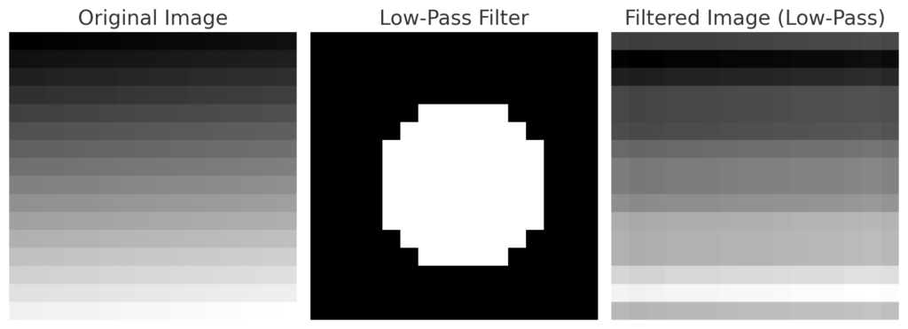
Here is the plot showing the original image, the applied low-pass filter, and the filtered image:

1. Original Image: A synthetic gradient image.
2. Low-Pass Filter: The circular filter applied in the frequency domain.
3. Filtered Image: The result of applying the low-pass filter and performing the inverse FFT.

6. Complete Example: Noise Reduction in an Image

Here’s a complete example to tie everything together:

% Load the image
img = imread('cameraman.tif');

% Perform FFT
fft_result = fft2(img);
fft_shifted = fftshift(fft_result);

% Create a low-pass filter
[m, n] = size(img);
[x, y] = meshgrid(-n/2:n/2-1, -m/2:m/2-1);
radius = sqrt(x.^2 + y.^2);
low_pass_filter = radius < 50;

% Apply the filter
filtered_fft = fft_shifted .* low_pass_filter;

% Perform the inverse FFT
filtered_img = ifft2(ifftshift(filtered_fft));

% Display results
subplot(1, 3, 1); imshow(img); title('Original Image');
subplot(1, 3, 2); imshow(log(1 + abs(fft_shifted)), []); title('Magnitude Spectrum');
subplot(1, 3, 3); imshow(uint8(real(filtered_img))); title('Filtered Image');

This example demonstrates how to reduce noise using a low-pass filter, making the output image clearer.

Learn MATLAB with Online Tutorials

Explore our MATLAB Online Tutorial, your ultimate guide to mastering MATLAB! Whether you’re a beginner or an advanced user, this guide covers everything from basic MATLAB concepts to advanced topics

Interpreting fft2 Results: Spectral Analysis

Interpreting the results obtained from the FFT2 function in MATLAB is crucial for individuals engaged in spectral analysis. Through FFT2, one can transform a two-dimensional signal into the frequency domain, providing insights into its frequency characteristics. This transformation aids in identifying dominant frequency components present in the data, allowing for a more nuanced understanding of the underlying signal.

The frequency domain representation generated by FFT2 consists of complex numbers, which can be visualized using various techniques. A common approach is to compute the magnitude and phase spectra. The magnitude spectrum highlights the amplitude of each frequency component, while the phase spectrum indicates the phase shift associated with these components. By plotting the magnitude spectrum, practitioners can easily discern significant frequency components and their relative amplitudes.

When analyzing the FFT2 results, it is essential to understand how to interpret the output matrix. Each element in the resulting matrix corresponds to a frequency pair, where the row index represents the vertical frequency and the column index correlates to the horizontal frequency. It is also important to utilize techniques such as log-scaling when visualizing the data. Logarithmic scaling can provide a clearer picture of both low and high magnitude components, making it easier to identify important features within the spectrum.

However, there are common pitfalls to watch out for during spectral analysis. For instance, it is vital to ensure that the input data are pre-processed correctly, as this can heavily influence the results. Removing noise and applying windowing techniques can improve accuracy. Best practices include understanding the Nyquist theorem to avoid aliasing and carefully selecting the window size to optimize frequency resolution. By adhering to these guidelines, data scientists can enhance their ability to interpret FFT2 results effectively, leading to more reliable conclusions from spectral analyses.

Optimizing fft2 Performance in MATLAB

Optimizing the performance of the FFT2 function in MATLAB is crucial for data scientists and programmers who handle large datasets and require efficient computational methods. The FFT2 function, which computes the 2-dimensional fast Fourier transform, demands a careful approach to minimize computational complexity and maximize processing speed.

One primary strategy for enhancing FFT2 performance is to utilize MATLAB’s built-in functions effectively. MATLAB is optimized for performance, and functions like fft2 are implemented in a way that leverages low-level optimizations. To achieve optimal performance, it is recommended to ensure that the input data is appropriately sized and structured. For instance, dimensions of the input matrix should ideally be powers of two, which facilitates faster calculations by the FFT2 algorithm.

Another key aspect of optimizing FFT2 involves parallel processing. MATLAB provides built-in support for concurrent execution through the Parallel Computing Toolbox, which allows users to distribute FFT2 computations across multiple cores or even machines. By partitioning data and executing parallel FFT2 operations, processing times can be significantly reduced, particularly when working with extensive datasets. Users can implement parallelism easily by utilizing the parfor function, which automatically spreads the computations over available processors.

Memory management also plays a pivotal role in optimizing FFT2 operations. Allocating memory efficiently and ensuring that the workspace does not become overly cluttered can enhance performance. MATLAB’s memory management practices involve preallocating matrices and using logical indexing instead of resizing matrices dynamically. Such practices reduce overhead and improve memory access speed, enhancing the overall performance of the FFT2 function.

In summary, achieving optimal performance for FFT2 in MATLAB necessitates a multifaceted approach that includes using built-in functions wisely, applying parallel processing techniques, and managing memory efficiently. By considering these factors, programmers and data scientists can maximize their efficiency when processing complex datasets with FFT2.

Common Challenges and Troubleshooting fft2 in MATLAB

The Fast Fourier Transform (FFT) function is pivotal in analyzing frequency components in signal processing, and its two-dimensional variant, FFT2, extends its applicability to matrices and images. However, users frequently encounter various challenges when implementing FFT2 in MATLAB. Understanding these issues is crucial for effective troubleshooting and can significantly enhance the data analysis experience.

One common challenge arises from input size mismatches. FFT2 expects input data to be in the form of a matrix. If the matrix is not well-formed or contains non-numeric values, MATLAB will return an error. To avoid this, ensure that your data is correctly formatted and that all elements are numeric before applying the FFT2 function. Additionally, it is beneficial to check for the presence of NaN or Inf values, as these can disrupt the calculation.

Another issue often faced by users is related to computational complexity. Since FFT2 executes in O(N log N) time, large matrices can lead to significant computation times or memory overload. To mitigate this, consider down-sampling your data or employing more efficient algorithms tailored for large datasets. This strategy not only speeds up processing but also maintains the integrity of the frequency components being analyzed.

Furthermore, users should be on the lookout for specific error messages. For instance, the error “Too many input arguments” typically indicates that the function has been incorrectly called. A practical approach here is to consult MATLAB’s documentation for correct syntax usage. Additionally, ensuring that all required toolboxes are installed can help circumvent missing function errors.

In conclusion, while the FFT2 function in MATLAB offers remarkable capabilities for data analysis, users must be aware of potential challenges. By understanding common errors, ensuring proper data formatting, and optimizing matrix sizes, one can effectively troubleshoot and utilize FFT2 to its full potential.

Conclusion and Future Directions in FFT Analysis

In conclusion, mastering FFT2 in MATLAB is crucial for data scientists and programmers who aim to efficiently analyze complex data sets. The ability to transform data from the time domain to the frequency domain provides invaluable insights across various fields, including engineering, telecommunications, biomedical research, and more. Through this comprehensive guide, readers have gained an understanding of the foundational principles of FFT analysis, practical implementation strategies, and advanced techniques for optimizing performance. Emphasizing the importance of FFT2 specifically, it is evident that this tool not only streamlines data processing but also enhances the accuracy of frequency analysis.

Looking ahead, the landscape of signal processing is poised for evolution. The continuous advancement of computational technologies is likely to introduce more refined algorithms and techniques, potentially shifting the focus towards faster and more efficient alternatives to traditional FFT methods. For instance, methods like the Fast Wavelet Transform (FWT) and other multi-resolution techniques are gaining traction as they allow for localized frequency analysis, offering advantages in analyzing non-stationary signals or time-varying data.

Moreover, the integration of machine learning and artificial intelligence with FFT analysis hints at an exciting frontier. By harnessing the power of data-driven models, it is possible to uncover patterns and features in data that standard FFT techniques might overlook. As data sets become increasingly large and complex, exploring these hybrid approaches may open new avenues for insights and discovery in various applications.

As you continue your journey in mastering FFT2 within MATLAB, staying informed about upcoming trends and technologies will be essential. The future of FFT analysis signifies not only the relevance of this powerful technique but also the opening of doors to innovative approaches, ultimately transforming how data is interpreted and utilized across disciplines.

Other Functions in MATLAB

MATLAB Ode45 function – Practical Tutorials

Ode45 is a widely utilized numerical solver designed for the effective resolution of ordinary differential equations (ODEs). It is a part of MATLAB’s ODE suite and is specifically tailored to handle problems where the solution requires the calculation of derivatives at multiple points. The significance of Ode45 stems from its implementation of the Runge-Kutta method, which offers a robust approach to approximating solutions with high accuracy.

MATLAB Diff function – Beginners Tutorials

MATLAB diff function is an essential tool utilized in the realms of data analysis and programming. Primarily, it calculates the differences between adjacent elements in an array, offering valuable insights into trends and behaviors of data sets. Through a blend of theoretical understanding and hands-on practical examples, this guide aspires to empower readers to utilize MATLAB’s diff effectively, transforming raw data into actionable insights.

MATLAB conv2 Function

Convolution is a mathematical operation that combines two functions to produce a third function, expressing how the shape of one function is modified by the other. Convolution is calculated using MATLAB conv2 function. This operation is particularly crucial in various fields such as image processing, signal analysis, and systems engineering. This function is specifically designed for two-dimensional convolution, making it preferable for tasks that involve images or other matrix-based data

MATLAB interp1 Function

The interp1 function in MATLAB serves as a fundamental tool for conducting one-dimensional interpolation on a set of data points. Interpolation is a statistical method that estimates values between two known values, allowing for more precise data analysis and management. By employing the interp1 function, users can obtain interpolated values at specified points, thus enabling a deeper analysis of datasets.

fzero MATLAB Function

The fzero in MATLAB is a powerful tool designed for finding the roots of nonlinear equations. This function plays a crucial role in various fields, including engineering, data science, and mathematical modeling. By utilizing fzero MATLAB, users can efficiently identify points where a given function equals zero, which is essential for solving problems that involve polynomial equations, differential equations, and optimization tasks.