Introduction to Gradient Descent
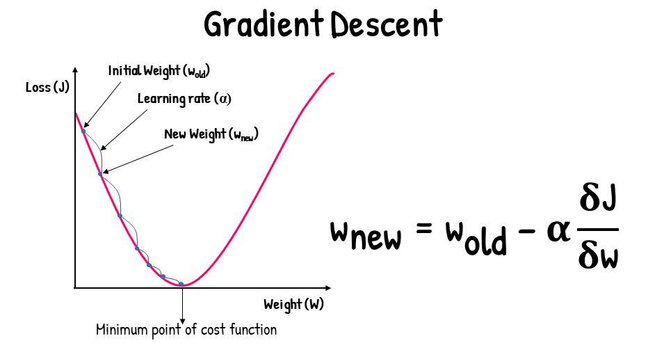
Gradient descent is an iterative optimization algorithm widely used in machine learning and statistical modeling, primarily for minimizing cost functions. This method is pivotal in various applications, including linear regression, logistic regression, and neural network training. At its core, GD focuses on finding the minimum of a function by iteratively moving in the direction of the steepest descent, which is mathematically represented by the negative gradient of the function.
The process begins with an initial guess or point in the parameter space. The gradient, which is essentially the vector of partial derivatives, provides insight into how the function changes with respect to each parameter. By calculating the gradient, one determines the direction that the parameters need to be adjusted to reduce the function’s value. The adjustment is controlled by a so-called learning rate, a hyperparameter that dictates the size of the steps taken towards the minimum.
In the context of machine learning, the significance of gradient descent lies in its effectiveness to optimize complex models by reducing the error between predicted and actual outcomes. When applied in Python, users can leverage libraries such as NumPy and TensorFlow to implement the gradient descent algorithm efficiently. Such implementations streamline the process, allowing practitioners to focus on model tuning rather than intricate calculations. Furthermore, gradient descent comes in various forms, including batch, stochastic, and mini-batch, each suitable for different datasets and use cases.
Understanding the principles behind gradient descent is essential for mastering machine learning, as it serves as the backbone for many algorithms used today. Its ability to navigate the parameter space makes it a fundamental tool that every data scientist should be familiar with when working on optimization problems in Python.
The Mathematics Behind Gradient Descent
At the core of the gradient descent algorithm lies an important mathematical concept known as the derivative. The derivative of a function at a particular point provides information about the slope or rate of change at that specific point. In the context of optimization, understanding the derivative is crucial, as it allows one to determine how to move towards a minimum or maximum of a function.
Stochastic Gradient Descent (SGD) is grounded in the principles of optimization, specifically tailored for minimizing a loss function, which quantifies the discrepancy between the predicted values produced by a model and the actual target values. In mathematical terms, consider a common formulation where we aim to minimize a loss function L(theta), where theta represents parameters that we are trying to optimize. The objective typically consists of finding the optimal parameters that minimize this loss across a dataset.
1. The Objective of SGD
The goal of SGD is to find optimal parameters that minimize a given loss function. Mathematically, we aim to minimize:
L(θ)where θ represents the parameters being optimized.
2. Role of Gradients in SGD
The core of SGD lies in the calculation of gradients, which are essential to direct the parameter updates. For a given iteration, SGD introduces randomness by selecting a subset of data, known as a mini-batch, instead of utilizing the complete dataset. The gradient of the loss function with respect to the parameters is computed as follows:
∇L(θ) = (1/m) * Σ ∇l(yᵢ, f(xᵢ, θ))where:
mis the number of samples in the mini-batch.yᵢis the actual label.f(xᵢ, θ)is the predicted output by the model.ldenotes the individual loss function.
3. The Update Rule
The learning rate η plays a pivotal role as it determines the step size for each update. The updating rule in SGD can be articulated as:
θ ← θ - η ∇L(θ)This equation illustrates that the parameters are adjusted in the direction opposite to the gradient, scaled by the learning rate.
4. Importance of Learning Rate
The choice of learning rate significantly influences the performance of SGD:
- Too small: Slow convergence.
- Too large: Possible divergence.
The mathematics behind SGD thus emphasizes balancing these elements effectively to achieve efficient optimization in machine learning models.
5. Significance of SGD in Machine Learning
SGD is widely used in deep learning and other machine learning models because it efficiently updates parameters with lower computational cost compared to full-batch gradient descent.
By leveraging mini-batches and a well-chosen learning rate, SGD ensures rapid and effective optimization in various machine learning tasks.
There are various types of gradients that one may encounter, depending on the nature of the function. The most common are the steepest descent and stochastic gradients. The steepest descent method uses full information from the function’s gradient, while stochastic gradient descent (SGD) incorporates randomness by estimating the gradient from a sample of data points. Each type of gradient has its implications in the context of optimizing functions and their choice affects the convergence speed and stability of the gradient descent algorithm in Python.
Implementing Gradient Descent in Python
To begin implementing the gradient descent algorithm in Python, it is essential to first understand the underlying mathematics. Gradient descent is an optimization algorithm used to minimize a function by iteratively moving towards the steepest descent as defined by the negative of the gradient. Here’s a simple example to illustrate how to create a gradient descent algorithm in Python.
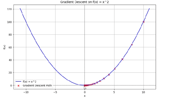
Let’s assume we want to minimize a simple quadratic function: f(x) = x^2. The gradient of this function, df/dx, is 2x. Our goal is to start from an initial guess and iteratively update our guess to converge to the optimum.
We can achieve this by following these steps:
1. Importing Required Libraries
We begin by importing the necessary libraries for numerical computation and visualization:
import numpy as np
import matplotlib.pyplot as plt
2. Defining the Function and Its Gradient
We define the quadratic function that we aim to minimize and its gradient:
def f(x):
    """Quadratic function f(x) = x^2"""
    return x ** 2

def gradient(x):
    """Gradient of the function f'(x) = 2x"""
    return 2 * x
This function represents a parabola with its minimum at x = 0. The gradient f'(x) = 2x tells us the direction of steepest ascent.
3. Implementing the Gradient Descent Algorithm
We define the gradient descent function that tracks the optimization path:
def gradient_descent(starting_point, learning_rate, num_iterations):
    """Perform gradient descent to minimize the function f(x)"""
    x_old = starting_point  # initial value
    x_history = [starting_point]  # Store history of x values for plotting

    for i in range(num_iterations):
        x_new = x_old - learning_rate * gradient(x_old)  # update x using the gradient
        x_history.append(x_new)  # Record new x value
        x_old = x_new  # update x_old for the next iteration

    return x_new, x_history
This enhanced version:
- Takes the same three parameters (starting point, learning rate, iterations)
- Maintains a history of all x values during optimization
- Returns both the final x value and the optimization path
4. Setting Parameters and Running Gradient Descent
We configure and execute the gradient descent:
# Parameters for gradient descent
starting_point = 10  # Starting point
learning_rate = 0.1  # Learning rate
num_iterations = 50  # Number of iterations

# Run gradient descent
min_x, history = gradient_descent(starting_point, learning_rate, num_iterations)

# Print results
print(f"Minimum value of x: {min_x:.2f}")
print(f"Function value at minimum: {f(min_x):.2f}")
5. Visualizing the Optimization Process
We create a visualization showing both the function and the optimization path:
# Generate x values for plotting the function
x_values = np.linspace(-11, 11, 100)
y_values = f(x_values)

# Plotting the function and the gradient descent path
plt.figure(figsize=(10, 6))
plt.plot(x_values, y_values, label='f(x) = x^2', color='blue')
plt.scatter(history, f(np.array(history)), color='red', label='Gradient Descent Path', marker='x')
plt.title('Gradient Descent on f(x) = x^2')
plt.xlabel('x')
plt.ylabel('f(x)')
plt.axhline(0, color='black', linewidth=0.5, linestyle='--')
plt.axvline(0, color='black', linewidth=0.5, linestyle='--')
plt.legend()
plt.grid()
plt.show()
6. Key Improvements in This Implementation
- Visualization: Shows the complete optimization path on the function curve
- Tracking: Maintains history of all intermediate x values
- Precision: Uses formatted output for clearer results
- Documentation: Includes docstrings for better code understanding
The visualization demonstrates how gradient descent navigates from the starting point (x=10) down to the minimum (x≈0), with each iteration marked by a red ‘x’. The learning rate of 0.1 ensures stable convergence without overshooting.
Complete SDG Code in Python
import numpy as np
import matplotlib.pyplot as plt

# Function Definitions
def f(x):
    """Quadratic function f(x) = x^2"""
    return x ** 2

def gradient(x):
    """Gradient of the function f'(x) = 2x"""
    return 2 * x

# Gradient Descent Algorithm
def gradient_descent(starting_point, learning_rate, num_iterations):
    """Perform gradient descent to minimize the function f(x)"""
    x_old = starting_point  # initial value
    x_history = [starting_point]  # Store history of x values for plotting

    for i in range(num_iterations):
        x_new = x_old - learning_rate * gradient(x_old)  # update x using the gradient
        x_history.append(x_new)  # Record new x value
        x_old = x_new  # update x_old for the next iteration

    return x_new, x_history

# Main Execution
# Parameters for gradient descent
starting_point = 10  # Starting point
learning_rate = 0.1  # Learning rate
num_iterations = 50  # Number of iterations

# Run gradient descent
min_x, history = gradient_descent(starting_point, learning_rate, num_iterations)

# Print results
print(f"Minimum value of x: {min_x:.2f}")
print(f"Function value at minimum: {f(min_x):.2f}")

# Visualization
# Generate x values for plotting the function
x_values = np.linspace(-11, 11, 100)
y_values = f(x_values)

# Plotting the function and the gradient descent path
plt.figure(figsize=(10, 6))
plt.plot(x_values, y_values, label='f(x) = x^2', color='blue')
plt.scatter(history, f(np.array(history)), color='red', label='Gradient Descent Path', marker='x')
plt.title('Gradient Descent on f(x) = x^2')
plt.xlabel('x')
plt.ylabel('f(x)')
plt.axhline(0, color='black', linewidth=0.5, linestyle='--')
plt.axvline(0, color='black', linewidth=0.5, linestyle='--')
plt.legend()
plt.grid()
plt.show()
In this example, we define the function along with its gradient. The gradient_descent function takes a starting point, learning rate, and the number of iterations as inputs, and iteratively updates the position to find the minimum. After executing the code, we find that the variable minimum_x converges towards zero, demonstrating that our gradient descent implementation in Python is functioning correctly. This simple example serves as a foundational understanding of how to write your own gradient descent algorithm from scratch, allowing you to explore more complex functions and datasets.
Types of Gradient Descent
Gradient descent is a widely used optimization algorithm in machine learning and statistical modeling. It is essential to understand the different types of gradient descent methods, as each has unique characteristics that suit varying datasets and objectives. The three primary types of gradient descent include batch gradient descent, SGD, and mini-batch GD.
Batch gradient descent calculates the gradient of the cost function with respect to the parameters for the entire training dataset. This method ensures a smooth and thorough update of parameters but can be computationally expensive and slow, particularly for large datasets. When implementing gradient descent in Python using this approach, users often face challenges with memory usage and training time. However, the convergence is stable and less noisy, making it suitable for simpler models where the entire dataset can be processed at once.
In contrast, SGD, updates the parameters using only one training example at each iteration. This approach drastically reduces computation time and can lead to faster convergence. However, it introduces a level of noise in the gradient estimates, which might hinder the final convergence. Implementing the gradient descent algorithm in Python with SGD can help to escape local minima quickly, making it an attractive option for complex models like neural networks that handle large volumes of data.
Lastly, mini-batch gradient descent strikes a balance between batch and stochastic methods. By using a small random sample of the training dataset to compute each update, mini-batch gradient descent combines the efficiency of SGD with the stability of batch gradient descent. It is particularly useful for handling large datasets where performance optimization is crucial. In conclusion, selecting the right gradient descent method ultimately depends on the specific requirements of the task, computational resources, and the nature of the dataset involved.
What is Stochastic Gradient Descent?
Stochastic Gradient Descent (SGD) is an optimization algorithm commonly employed in machine learning and deep learning to minimize the error in learning models. Unlike traditional gradient descent approaches, such as Batch Gradient Descent, which utilize the entire training dataset to compute the gradient of the loss function, SGD operates on one training example at a time. This allows for a more frequent update of model parameters, potentially leading to faster convergence, especially when dealing with large datasets.
One of the fundamental characteristics of SGD is its stochastic nature. By randomly selecting a single training example (or a small batch of examples) at each iteration, it introduces variability in the updates, which often helps the algorithm to escape local minima and explore the loss surface more effectively. This variability can lead to a more diverse set of solutions, although it may also cause the loss function to oscillate, making it harder to converge at times.
In comparison to Batch Gradient Descent, where all examples in the dataset influence the gradient calculation before making any parameter updates, SGD offers significant computational efficiency. Since it processes only one sample at a time, the algorithm can scale well with large datasets, allowing for quicker iterations through the training process. Moreover, the frequent updates enabled by SGD can lead to improved learning rates and more dynamic convergence behavior, which can be advantageous in practice.
However, the advantages of Stochastic Gradient Descent come with trade-offs; the noise introduced by its stochastic updates may require careful tuning of hyperparameters such as the learning rate and batch size. Overall, SGD represents a valuable approach in the field of machine learning, particularly when optimizing models over extensive datasets where performance and speed are critical considerations.
Choosing the Right Learning Rate
The learning rate is a critical hyperparameter in the gradient descent algorithm that dictates the size of the steps taken as the algorithm progresses to minimize the loss function. Choosing the right learning rate is essential for ensuring that the model converges efficiently without oscillating or converging too slowly. A learning rate that is too high can result in overshooting the minimum, causing divergence from the optimal solution, while a rate that is too low can lead to an excessively long training time and could potentially get stuck in local minima.
When implementing gradient descent in Python, it is common practice to experiment with various learning rates to observe their effects on the model’s performance. For example, a typical learning rate might start at 0.01, but depending on the dataset and specific algorithm, it can be adjusted higher or lower. It often helps to visualize the loss over iterations, which can reveal whether the chosen learning rate is effective. A learning rate that works well in one context may not be suitable for another, thus necessitating an iterative approach in finding the optimal value.
Additionally, several techniques can aid in managing learning rates effectively. Learning rate schedules, for instance, involve gradually decreasing the learning rate as the training progresses. This approach can provide large steps initially to expedite the convergence but allows finer adjustments later in training as the model approaches the minimum. Alternatively, adaptive learning rate methods such as Adam or RMSprop adjust the learning rate dynamically based on the gradients, which is a common practice in modern machine learning frameworks using Python. These methods are particularly useful for complex models and datasets, improving performance significantly in many gradient descent examples.
Overcoming Challenges
Gradient descent is a powerful optimization algorithm widely used in machine learning and deep learning applications. However, practitioners often encounter several challenges when implementing the gradient descent algorithm in Python. Understanding these challenges is essential for effective utilization of the technique.
One common issue is the possibility of getting stuck in local minima. Depending on the initialization of parameters, the gradient descent algorithm can converge to a point that is not the global minimum of the loss function. This can lead to suboptimal model performance. To mitigate this, techniques such as multiple initializations and the use of advanced optimizers can be employed. Using a gradient descent example that highlights random restarts can often yield better overall results.
Another frequent complication is oscillation, where the model fails to settle into a minimum due to improper learning rates. If the learning rate is set too high, it can cause the gradients to overshoot, leading to instability in convergence. To address this, practitioners can utilize techniques such as learning rate schedules, which adjust the learning rate over time, and momentum, which helps smooth out the oscillations by accumulating past gradients. This adjustment allows for a more refined search process within the parameter space.
Additionally, slow convergence remains a critical challenge, particularly in high-dimensional spaces. This can be exacerbated by poor feature scaling or inappropriate choices of the learning rate. Therefore, employing adaptive algorithms such as Adam or RMSprop, which adapt the learning rate based on parameter updates, can dramatically accelerate convergence. These adjustments create a more responsive gradient descent in Python, allowing it to navigate the loss landscape more efficiently.
By recognizing these potential challenges and applying the suggested strategies, users can enhance their experience with the gradient descent algorithm in Python, leading to more effective and efficient model training.
Need Help in Programming?
I provide freelance expertise in data analysis, machine learning, deep learning, LLMs, regression models, NLP, and numerical methods using Python, R Studio, MATLAB, SQL, Tableau, or Power BI. Feel free to contact me for collaboration or assistance!
Follow on Social

Applications of Gradient Descent
Gradient descent serves as a fundamental optimization algorithm widely applied across various domains, particularly in machine learning, deep learning, and artificial intelligence. Its capability to minimize loss functions makes it an invaluable tool for training models effectively. In machine learning, for instance, GD is prominently used in linear regression. The algorithm iteratively adjusts the model parameters to reduce the difference between predicted and actual values, ultimately enabling the creation of reliable prediction models.
In the realm of deep learning, gradient descent plays a critical role in optimizing neural networks. Here, it is employed to fine-tune weights considering the vast complexity of layered architectures. By utilizing techniques such as mini-batch or stochastic gradient descent, practitioners streamline the training process, achieving faster convergence and enhancing the model’s accuracy. The flexibility of GD in Python allows developers to implement these varied methodologies efficiently, catering to specific problem domains.
Another noteworthy application is in artificial intelligence systems, where gradient descent is integral for reinforcement learning algorithms. Through this approach, agents learn optimal strategies by minimizing the expected error between predicted outcomes and actual rewards, leading to improved decision-making capabilities in dynamic environments. Moreover, gradient descent is beneficial in fields like computer vision and natural language processing, where it optimizes feature extraction and enhances model performance. For instance, in image classification tasks, convolutional neural networks utilize gradient descent to adjust filter weights, thereby elevating classification accuracy.
In summary, the versatility of the gradient GD in Python enables its application across diverse fields. This not only exemplifies its importance in training and optimizing models but also underscores the ever-growing relevance of gradient descent in the development of advanced AI technologies.
Comparing Gradient Descent with Other Optimization Algorithms
Gradient descent is one of the most widely adopted optimization algorithms in machine learning and deep learning fields. However, it is essential to consider how it compares to other optimization techniques like Newton’s method, genetic algorithms, and various optimization libraries. Each approach has its own advantages and disadvantages, which can influence the choice of method in specific contexts.
To begin with, Newton’s method is a second-order optimization technique that can converge quickly, using the Hessian matrix to consider curvature. This often allows it to find the local minimum with fewer iterations compared to gradient descent. However, Newton’s method has its limitations, as it is computationally expensive in terms of memory and processing power, especially for large datasets, where evaluating the Hessian matrix can become infeasible. Consequently, while Newton’s method may provide more accuracy in certain scenarios, it is not typically the first choice when implementing gradient descent in Python due to its inherent complexity.
On the other hand, genetic algorithms represent a family of optimization techniques inspired by the process of natural selection. These algorithms involve populations and generations to search for solutions. While genetic algorithms can be effective in finding global optima, they require careful tuning and are generally slower than gradient descent. The random nature of genetic algorithms might lead to less consistent outcomes compared to a deterministic gradient descent example, making them less suitable for scenarios with strict convergence requirements.
Similarly, various optimization libraries, such as SciPy and TensorFlow, offer robust implementations of gradient descent and other algorithms. These libraries often incorporate advanced features such as adaptive learning rates and momentum methods, which can enhance the performance of the gradient descent algorithm in Python. Nevertheless, the choice of an optimization algorithm should depend on the specific characteristics of the problem at hand, alongside considerations of computational efficiency and accuracy. In conclusion, understanding these alternatives—Newton’s method, genetic algorithms, and optimization libraries—can provide valuable insights into when to effectively utilize gradient descent versus other methods in Python, ensuring the most optimal outcomes in a range of applications.
Learn Python for Data Analysis Assignment
This guide offers a thorough introduction to Python, presenting a comprehensive guide tailored for beginners who are eager to embark on their journey of learning Python from the ground up.

Conclusion and Future Directions
In this blog post, we have explored the concept of GD in Python, a fundamental optimization technique used in various machine learning algorithms. We began by defining the gradient descent algorithm, explaining its importance in minimizing error functions through iterative updates of parameters. As we delved deeper, we provided practical examples to illustrate the implementation of gradient descent in Python. These included discussions on key variations of the algorithm, such as stochastic GD, as well as the significance of learning rate selection in achieving convergence.
Given the rising complexity of data and models in machine learning, the applications of GD techniques continue to evolve. Future research in this area may focus on improving the efficiency of the gradient descent algorithm in Python, including innovations in adaptive learning rates and the use of advanced optimization techniques such as momentum and Nesterov accelerated GD. Researchers may also explore hybrid approaches that combine GD with other optimization algorithms to enhance convergence rates and find better local minima.
Moreover, the integration of GD in deep learning frameworks has opened new avenues for exploration. As practitioners experiment with larger datasets and more complex architectures, it will be vital to investigate the implications of GD on performance and computational resources. For those venturing into applied machine learning projects, we encourage continued experimentation with GD in Python. Engaging with various datasets, tweaking hyperparameters, and observing the outcomes will deepen your understanding of this crucial algorithm.
In conclusion, gradient descent remains a cornerstone of optimization techniques in machine learning. By grasping its underlying principles and potential future developments, you will be well-equipped to leverage gradient descent and enhance your own projects.