Introduction to the Finite Element Method
The Finite Element Method (FEM) is a powerful numerical technique used to obtain approximate solutions to boundary value problems for partial differential equations. Initially developed in the 1950s for use in structural engineering, FEM has since revolutionized the analysis of complex physical systems across various fields, including mechanical, civil, and aerospace engineering, as well as in physics and bioengineering and its easy to implement Finite Element Method in MATLAB. Its versatility and efficacy have made it a vital tool for engineers and scientists alike.
At its core, the finite element method involves breaking down a large, complex problem into smaller, more manageable parts known as finite elements. This decomposition allows for the simplification of complex geometries and boundary conditions, enabling more straightforward computation. Each element is then analyzed collectively to determine a solution to the overall problem. The process generally begins with the discretization of a domain, followed by the formulation of element equations, and culminates in the assembly of a global system of equations that can be solved using various numerical methods.
Many types of problems can be solved using FEM, including linear and nonlinear structural analysis, heat transfer, fluid dynamics, and electromagnetics. The flexibility of this method allows it to be adapted for both static and dynamic analyses, making it suitable for a wide range of engineering challenges. Moreover, the ability to implement the finite element method in MATLAB has further enhanced its accessibility, as MATLAB provides a user-friendly platform for performing finite element analysis in MATLAB. With the extensive resources available for finite element analysis in MATLAB, such as specialized toolboxes and libraries, users can effectively and efficiently apply FEM to their projects.
In conclusion, the Finite Element Method stands as a crucial development in the field of numerical analysis, enabling the resolution of complex engineering problems through systematic decomposition and solution assembly. It is essential for practitioners to grasp the fundamental principles of FEM, as well as its applications and implementation within platforms like MATLAB.

Key Concepts of FEM
The Finite Element Method (FEM) is a powerful numerical technique used to solve complex engineering problems, particularly in structural analysis and computational physics. At the heart of FEM are several key concepts that are essential for understanding its methodology. One of the foremost concepts is discretization, which involves dividing a continuous domain into smaller, manageable elements. This process transforms a complex physical problem into a simpler mathematical representation, which can then be solved more effectively using finite element analysis in MATLAB.
Another critical aspect of FEM is the use of shape functions. These polynomial functions are defined over each element and are instrumental in approximating the field variables within the elements. By using shape functions, we can interpolate values of the variables based on the nodal values, enabling a smooth approximation of the solution across the entire domain. The accuracy of the FEM solution is significantly influenced by the choice of these shape functions and their corresponding degree.
The assembly of global matrices is another vital concept. As individual elements are analyzed to yield local stiffness or mass matrices, these components must be assembled into a global system that reflects the entire domain’s behavior. This step is crucial, as it captures the interaction between different elements. In practical applications with FEA in MATLAB, this assembly process is accomplished using efficient algorithms to ensure that the computational effort remains manageable, even for large-scale problems.
Lastly, boundary conditions play a significant role in FEM. These conditions define how the system interacts with its environment and include displacements, forces, or other constraints applied to the boundary of the domain. Properly applying boundary conditions is essential for obtaining accurate solutions in finite element method MATLAB implementations. Understanding these fundamental concepts will provide a solid groundwork for anyone looking to apply finite element method with MATLAB in practical or research scenarios.
Setting Up MATLAB for FEM Analysis
Preparing your MATLAB environment for finite element analysis is the first crucial step toward successful implementation of the finite element method (FEM) in MATLAB. To effectively conduct FEM analysis, it is essential to ensure that you have the appropriate toolboxes and resources at your disposal. The primary toolbox required for such simulations is the Partial Differential Equation Toolbox, which provides essential functions for modeling and solving PDEs using the finite element method.
Once you have installed the necessary toolboxes, launching MATLAB will present a user interface that is conducive to setting up finite element problems. Users should familiarize themselves with the various panels, such as the Command Window, where commands can be entered; the Workspace, which allows tracking of variable states; and the Editor, where scripts can be created and edited. It is recommended to create a new project that encapsulates all components of your finite element model. To create a new project, navigate to the Home tab, select “New,” and then “Project.” This helps in organizing your files and analyses, especially when dealing with complex FEM in MATLAB applications.
In addition to the standard toolboxes, there are various resources and libraries available that augment the capabilities of FEM in MATLAB. Numerous open-source frameworks, such as FEniCS and FreeFEM, can be integrated for extended functionalities or specific applications. Additionally, MATLAB offers extensive resources, including tutorials and documentation, which can assist in familiarizing yourself with the finite element method with MATLAB. Online forums and MATLAB Central can also serve as valuable platforms for exchanging ideas and seeking assistance regarding specific finite element analysis challenges.
Meet Ahsan – Certified Data Scientist with 5+ Years of Programming Expertise
👨💻 I’m Ahsan — a programmer, data scientist, and educator with over 5 years of hands-on experience in solving real-world problems using: Python, MATLAB, R, SQL, Tableau and Excel
📚 With a Master’s in Engineering and a passion for teaching, I’ve helped countless students and researchers: Complete assignments and thesis coding parts, Understand complex programming concepts, Visualize and present data effectively
📺 I also run a growing YouTube channel — Algorithm Minds, where I share tutorials and walkthroughs to make programming easier and more accessible. I also offer freelance services on Fiverr and Upwork, helping clients with data analysis, coding tasks, and research projects.
Contact me at
📩 Email: ahsankhurramengr@gmail.com
📱 WhatsApp: +1 718-905-6406

Why Clients Trust Me – Real Stories, Real Results

“Ahsan completed the project sooner than expected and was even able to offer suggestions as to how to make the code that I asked for better, in order to more easily achieve my goals. He also offered me a complementary tutorial to walk me through what was done. He is knowledgeable about a range of languages, which I feel allowed him to translate what I needed well. The product I received was exactly what I wanted and more.” 🔗 Read this review on Fiverr
Katelynn B.
Implementing Finite Element Method in MATLAB: A Step-by-Step Tutorial and Complete Code
The Finite Element Method (FEM) is a powerful computational technique widely used for engineering and scientific applications. In MATLAB, the implementation of FEM can be achieved efficiently with a systematic approach. This tutorial will walk you through the essential steps to implement a finite element analysis in MATLAB, making it accessible for both beginners and those with prior experience.
FEM MATLAB Complete Code
% Parameters
L = 20;                    % Length of the rod
N = 20;                    % Number of grid points
alpha = 0.1;              % Thermal diffusivity
T0 = 300;                  % Initial temperature at the left boundary
TL = 0;                    % Initial temperature at the right boundary
t_end = 50;                 % End time
dx = L / (N - 1);          % Spatial step size
dt = 0.5;               % Time step size

% Stability condition check
if alpha * dt / dx^2 > 0.5
    error('Time step is too large, stability condition not satisfied.');
end

% Initial temperature distribution (example: linear profile)
x = linspace(0, L, N);     % Spatial grid
T = ones(1, N).*TL;           % Initialize with zero temperature everywhere
T(1) = T0;                 % Set the left boundary temperature

% Initializing figure for animation (optional)
figure;

% Time-stepping loop
for t = 0:dt:t_end
    % Create a copy of the current temperature distribution
    T_new = T;

    % Loop over all grid points (excluding boundaries)
    for i = 2:N-1
        T_new(i) = T(i) + (alpha * dt / dx^2) * (T(i-1) - 2*T(i) + T(i+1));
    end

    % Update the temperature profile
    T = T_new;

    % Apply boundary conditions
    T(1) = T0;     % Left boundary
    T(N) = TL;     % Right boundary

    % Plot the current temperature distribution
    plot(x, T, '-o');
    title(sprintf('Time = %.2f seconds', t));
    xlabel('Position (x)');
    ylabel('Temperature (T)');
    axis([0 L 0 300]);
    pause(0.1);  % Pause to update the plot (for animation)
end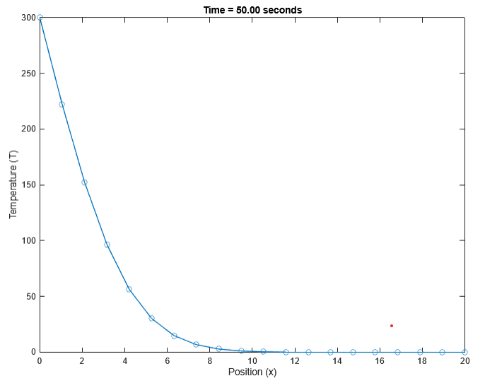
We begin by defining the problem geometry. This can involve specifying points, lines, and surfaces that represent the physical domain of interest. Depending on your application, you might use predefined functions in MATLAB or create custom definitions. Once the geometry is established, the next step is to assign material properties. These properties include elastic modulus, density, and Poisson’s ratio, which influence how the material behaves under loads. In MATLAB, these properties can be easily stored in data structures for easy access during the analysis.
Next, we discretize the geometry into finite elements. This process involves dividing the geometry into smaller subdomains (elements) where the equations will be solved. In MATLAB, you can construct the mesh using available functions or external mesh generators. Following this, we formulate the system of equations based on the finite element method using the assembly process, where contributions from each element are combined to form the global stiffness matrix.
Once the system is formulated, we should proceed to apply boundary conditions and loads. This step is crucial as it defines how the model interacts with its environment. With all parameters set, we can solve the system of equations using MATLAB’s solver functions. Lastly, the results can be visualized through various plotting functions available in MATLAB, allowing for an intuitive understanding of the phenomenon under study.
This step-by-step approach to implementing the finite element method in MATLAB equips users with the necessary skills to perform fea in matlab effectively. By following these guidelines, one can gain a solid foundation in performing finite element analysis in MATLAB.
Common Applications of FEM in Engineering
The Finite Element Method (FEM) offers powerful capabilities for solving engineering problems across various domains. Its versatility makes it an invaluable tool in fields such as structural, thermal, fluid, and electromagnetic analysis. By implementing finite element analysis in MATLAB, engineers can conduct simulations that lead to more effective designs and solutions.
In structural engineering, for instance, FEM is commonly used to analyze load-bearing structures such as bridges and buildings. Engineers can model the geometry and material properties of structures within MATLAB to predict how they will respond to various loads. A practical example includes the assessment of stress distribution in a steel beam under a uniform load, enabling designers to identify potential failure points early in the design process.
Thermal analysis is another significant application of FEM in MATLAB. Engineers often perform simulations to evaluate heat transfer in components such as engine blocks or electronic devices. By implementing the finite element method with MATLAB, one could determine temperature distribution and thermal conductivity, which is crucial for ensuring safety and efficiency in thermal systems.
In fluid dynamics, FEM is utilized to analyze fluid flow and related phenomena. For example, engineers can model the flow of air around an aircraft wing to optimize its aerodynamic properties. This application of finite element analysis in MATLAB allows for the visualization of pressure distribution and flow patterns, significantly aiding the design process.
Finally, electromagnetic analysis often employs FEM to simulate the behavior of electrical circuits and magnetic fields. For example, the design of electrical machines can leverage finite element analysis in MATLAB to optimize performance by analyzing the magnetic field distribution and minimizing losses.
These examples illustrate the broad applicability of FEM across various engineering sectors, showcasing how finite element method with MATLAB contributes to innovative solutions and enhanced design processes.
MATLAB Assignment Help
If you’re looking for MATLAB assignment help, you’re in the right place! I offer expert assistance with MATLAB homework help, covering everything from basic coding to complex simulations. Whether you need help with a MATLAB assignment, debugging code, or tackling advanced MATLAB assignments, I’ve got you covered.
Why Trust Me?
- Proven Track Record: Thousands of satisfied students have trusted me with their MATLAB projects.
- Experienced Tutor: Taught MATLAB programming to over 1,000 university students worldwide, spanning bachelor’s, master’s, and PhD levels through personalized sessions and academic support
- 100% Confidentiality: Your information is safe with us.
- Money-Back Guarantee: If you’re not satisfied, we offer a full refund
Advanced Techniques and Extensions of FEM
The finite element method (FEM) in MATLAB has evolved to incorporate a variety of advanced techniques, which significantly enhance its effectiveness in simulating complex engineering problems. Among these techniques, dynamic analysis, nonlinear problem-solving, and adaptive mesh refinement stand out as pivotal elements that broaden the applications of finite element analysis in MATLAB.
Dynamic analysis involves analyzing structures and systems subjected to time-dependent forces. In contrast to static analyses, dynamic analysis allows engineers to evaluate how structures behave under dynamic loading conditions, such as vibrations, impact, or seismic activities. Tools within finite element analysis in MATLAB are tailored for dynamic simulations, enabling users to apply various time integration methods to capture the dynamic response with substantial accuracy.
Nonlinear problems often challenge traditional linear assumptions within FEM applications. Nonlinear analyses consider material properties and geometric changes that may occur during loading. MATLAB provides specific functions and toolboxes that facilitate solving nonlinear equations, accommodating large deformations or complex material behaviors. By leveraging these capabilities in fea with MATLAB, engineers can develop more realistic models that mirror real-world scenarios.
Adaptive mesh refinement is another advanced technique that significantly impacts the accuracy and efficiency of finite element modeling. This method allows for the refinement of the element mesh based on the solution’s gradient, enabling a finer mesh in regions of high stress or strain while allowing coarser elements elsewhere. By implementing adaptive mesh strategies in finite element method with MATLAB, analysts can optimize computational resources while still achieving high fidelity results in their simulations.
In conclusion, incorporating advanced techniques such as dynamic analysis, tackling nonlinear problems, and employing adaptive mesh refinement in fea in MATLAB can substantially enhance the analysis precision and effectiveness of finite element models. These strategies allow engineers to approach more complicated problems in various fields, ultimately leading to better-designed and safer structures.
Learn MATLAB with Free Online Tutorials
Explore our MATLAB Online Tutorial, your ultimate guide to mastering MATLAB! his guide caters to both beginners and advanced users, covering everything from fundamental MATLAB concepts to more advanced topics.

Troubleshooting Common Issues in FEM Implementation
Implementing the finite element method (FEM) in MATLAB can present several challenges, particularly for those who are new to finite element analysis in MATLAB. Understanding potential problems and their solutions is essential to achieving accurate and reliable results in finite element analysis. One common issue encountered is convergence problems. Convergence issues often arise due to inadequate mesh refinement or inappropriate boundary conditions. To tackle this, it is advisable to perform grid sensitivity analyses to ensure that the mesh is fine enough to capture essential physics while avoiding excessive computational costs.
Another critical aspect is the quality of the mesh. Poor mesh quality can result in numerical instabilities, which can adversely affect the accuracy of the simulation. When working with FE models in MATLAB, users should ensure that the mesh elements are well-shaped and that the aspect ratios are acceptable. Tools such as MATLAB’s built-in mesh generation functions can assist users in creating high-quality meshes. Furthermore, it is advisable to visually inspect the mesh to catch any irregularities early in the process.
Numerical instabilities can also stem from inappropriate time-stepping methods in dynamic analyses or insufficient integration schemes. Users should carefully consider the time increment size and the order of the integration method used in simulations involving transient behaviors. Running a modal analysis prior to imposing dynamic loads can help identify such instabilities and provide insight into proper model adjustments.
In dealing with FEM in MATLAB, maintaining version compatibility of MATLAB toolboxes and ensuring that all necessary toolboxes are installed can prevent software-related issues. Additionally, users should consult the extensive MATLAB documentation and user community forums, where many users share their insights and solutions to problems encountered during finite element method implementations. By addressing these common challenges with targeted strategies, users can enhance their experience and results in finite element method with MATLAB.
Resources for Further Learning of Finite Element Method in MATLAB
To develop a solid understanding of the finite element method in MATLAB, it is essential to access quality resources that cover both the theoretical aspects and practical applications of finite element analysis in MATLAB. Here is a curated list of valuable resources that can guide learners ranging from beginners to advanced users.
Textbooks are a foundational resource for learning finite element methods. “The Finite Element Method: Linear Static and Dynamic Finite Element Analysis” by Thomas J.R. Hughes is highly regarded for its comprehensive coverage of both the mathematical theory and its implementation in software, including a focus on the finite element method with MATLAB. Additionally, “An Introduction to the Finite Element Method” by J. N. Reddy offers clear explanations and examples, making it particularly accessible for newcomers to the field.
Online courses also serve as an excellent platform for structured learning. Websites like Coursera and edX offer courses specifically focused on finite element analysis in MATLAB. These courses often include video lectures, interactive exercises, and projects that allow learners to apply their knowledge in real-world scenarios. Additionally, the official MathWorks website provides a wealth of documentation and examples for using FEM in MATLAB, enabling users to learn directly from the source.
Furthermore, there are numerous academic articles and research papers available through platforms such as Google Scholar and ResearchGate. These publications delve into advanced concepts and recent developments in finite element methods, offering insights into how FEM in MATLAB is applied in various fields, including engineering and physics.
In conclusion, engaging with a variety of resources—including textbooks, online courses, and scholarly articles—will significantly enhance one’s understanding of finite element analysis in MATLAB. Continuous learning and exploration are crucial for mastering the finite element method and its practical implementation in diverse applications.
Conclusion: finite element method in MATLAB
In this exploration of the finite element method in MATLAB, we have delved deeply into its principles and applications, showcasing how this powerful tool is utilized for finite element analysis in MATLAB. The finite element method, commonly referred to as FEM, offers a robust framework for solving complex engineering and physical problems. MATLAB enhances this process through its intuitive interface and comprehensive libraries, thereby allowing users to implement the finite element method with MATLAB efficiently.
Throughout the blog post, we have highlighted various aspects of FE analysis, including the formulation of problems, implementation strategies, and best practices for obtaining reliable results. The integration of finite element MATLAB capabilities, such as mesh generation and solution techniques, demonstrates the versatility of this method. By employing FEM in MATLAB, engineers and researchers can analyze structural, thermal, and fluid dynamics issues with greater accuracy and efficiency.
Understanding and mastering finite element analysis in MATLAB is crucial for professionals looking to innovate within their respective fields. The ability to effectively apply fem in MATLAB can enhance problem-solving capabilities and drive advancements in technology and engineering design. Furthermore, gaining proficiency in finite element method MATLAB processes allows users to explore more complex and practical scenarios, ultimately fostering a deeper understanding of the underlying physical phenomena.
As we conclude this guide, we encourage readers to engage with the finite element method and apply the knowledge acquired in MATLAB. Whether you are a student, researcher, or industry professional, the skills you’ve developed in finite element analysis with MATLAB will serve as an invaluable asset in addressing real-world challenges and advancing your career.