MATLAB interp1 Function – Beginners Guide

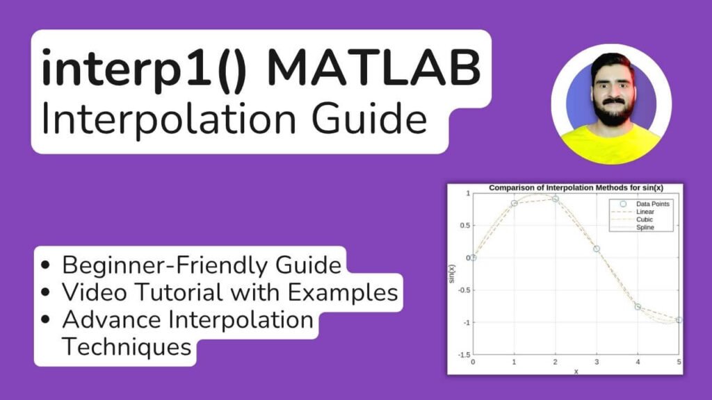
Introduction to interp1 MATLAB Function

The interp1 function in MATLAB serves as a fundamental tool for conducting one-dimensional interpolation on a set of data points. Interpolation is a statistical method that estimates values between two known values, allowing for more precise data analysis and management. Its significance lies in the ability to enhance data representation, which is particularly critical in fields such as engineering, scientific research, and finance, where accurate data interpretation is paramount. By employing the interp1 function, users can obtain interpolated values at specified points, thus enabling a deeper analysis of datasets.

MATLAB’s interp1 function operates on the premise that between any two points, there exists a continuum that can be approximated through various interpolation techniques such as linear, nearest neighbor, or spline methods. This flexibility makes it an invaluable resource for researchers and practitioners who must often work with incomplete datasets or who require high levels of accuracy in their computations. The syntax for the interp1 function is straightforward, which contributes to its user-friendliness. Typically, the function is called using the format: interp1(x, y, xi), where x and y are vectors representing the known data points, and xi is the point or points at which interpolation is desired.

In addition to the basic syntax, the interp1 function offers several options for interpolation methods, allowing users to tailor the function’s application to their specific needs. Understanding the function’s capabilities and variations can greatly empower users in analyzing and visualizing data. Thus, grasping the fundamentals of the interp1 function is essential for any MATLAB user looking to leverage the full potential of interpolation in their data analysis tasks.

Types of Interpolation Methods

The MATLAB interp1 function offers various interpolation methods, each with distinct characteristics suited to specific data types and desired outcomes. Understanding these methods is essential for selecting the most effective approach for your particular interpolation needs.

The first method is linear interpolation, which creates a straight line between two adjacent data points. This method is straightforward and efficient, often yielding satisfactory results for datasets where changes between points are approximately linear. However, it may not be suitable for cases with significant fluctuations or non-linear patterns, as it can oversimplify the data behavior.

Another method available within interp1 is nearest-neighbor interpolation. This technique assigns the value of the nearest data point to any point within the desired range. It is particularly useful for categorical data or when the original data is sparse, providing a quick solution. However, nearest-neighbor interpolation can lead to abrupt changes and may not smoothly represent the data trends.

Spline interpolation is a more advanced technique, utilizing polynomial functions to create a smooth curve that passes through all data points. This method is ideal for datasets that exhibit more complex behavior, as it minimizes oscillation problems associated with higher-degree polynomials. Spline interpolation is widely applicable in engineering and scientific fields where precise modeling is crucial.

Finally, cubic interpolation is often favored for its balance between complexity and accuracy. It employs cubic polynomials to generate a smooth transition between points while preserving local behavior. This method is valuable in scenarios where both smoothness and fidelity to the data trend are necessary, making it a popular choice for a diverse range of applications.

Preparing Data for interp1

When utilizing the MATLAB interp1 function for one-dimensional interpolation, the preparation of input data is crucial for obtaining accurate results. Specifically, the data must be organized into two vectors, x and y, which represent the dependent and independent variables, respectively. The vector x contains the data points at which the interpolation will be evaluated, while the vector y corresponds to the function values at those points.

To begin, it is essential to ensure that both x and y vectors are of equal length. The x vector should contain unique values, as duplicate entries may lead to ambiguities during the interpolation process. It is also important to organize the x values in ascending order. MATLAB’s interp1 function requires that the x vector is sorted, as the interpolation is performed based on the relationship between the x values and their corresponding y values. An unsorted x vector can result in errors or misleading interpolation results.

For instance, suppose we have the following data points: x = [1, 3, 2, 4] and y = [10, 30, 20, 40]. In this case, we first need to sort the x vector to get x = [1, 2, 3, 4] and adjust the y vector accordingly to y = [10, 20, 30, 40]. This restructuring ensures that the interp1 function accurately interpolates the data in a coherent manner. Additionally, it is advisable to consider the range of x values being used, as this will affect the interpolation accuracy when estimating values outside the manually defined x range.

In conclusion, preparing your data for the MATLAB interp1 function involves organizing x and y vectors effectively, checking for data redundancy, and ensuring proper sorting. Such a foundational step is vital to leverage the power of MATLAB for efficient and accurate interpolation. By following these guidelines, users can optimize the interpolation process and enhance their overall results.

Learn MATLAB with Online Tutorials

Explore our MATLAB Online Tutorial, your ultimate guide to mastering MATLAB! Whether you’re a beginner or an advanced user, this guide covers everything from basic MATLAB concepts to advanced topics

Step by Step Guide for interp1 in MATLAB

The interp1 function in MATLAB serves as a powerful tool for one-dimensional interpolation, allowing users to estimate values at intermediate points based on known data. Understanding its basic implementation is essential for anyone looking to analyze or manipulate datasets effectively using MATLAB. This section outlines the steps necessary to utilize interp1 through simple MATLAB examples.

In the simplest form, the syntax for interp1 is as follows:

yi = interp1(x, y, xi)

Here, x represents the original data points, y represents the corresponding values, and xi denotes the new data points at which interpolation is sought. The output, yi, contains the interpolated values corresponding to xi.

To illustrate, consider a basic example where data points are defined as:

x = [1, 2, 3, 4]
y = [10, 20, 30, 40]

If we want to interpolate values at new points, such as xi = [1.5, 2.5, 3.5], we can utilize the interp1 function as follows:

yi = interp1(x, y, xi);

The resulting output, yi, will contain the interpolated values at the specified points, demonstrating the ability of interp1 to estimate intermediate data effectively.

Moreover, MATLAB provides additional options to customize the interpolation method, such as linear, nearest, cubic, or spline. For example, specifying a linear interpolation can be done by adding a method parameter:

yi = interp1(x, y, xi, 'linear')

By exploring these different methods and utilizing the interp1 function, users can enhance their data analysis capabilities while ensuring accurate and visually appealing representations of their datasets.

This guide walks you through the function step by step, covering multiple interpolation methods, best practices, and troubleshooting tips. By the end, you’ll be able to apply interp1 to various real-world scenarios.

Getting Started: Prerequisites & Setup

Before diving into interpolation, ensure you have:

• MATLAB installed (R2016b or later recommended)
• Basic familiarity with vectors and plotting in MATLAB
• A dataset or sample data points to interpolate

To get started, define your known data points as vectors:

x = [0 1 2 3 4 5];  % Known x-values
y = [0 2 4 6 8 10]; % Corresponding y-values

These x and y values represent a linear relationship, but what if we need the value at x = 2.5? This is where interp1 comes in.

Interpolation Methods in interp1

MATLAB provides several interpolation methods. The syntax follows this pattern:

y_interp = interp1(x, y, xq, method);

Where:

• x, y → Known data points
• xq → Query points (where you need interpolated values)
• method → The interpolation technique (default is linear)

Linear Interpolation (Default)

Linear interpolation estimates values by connecting known points with straight lines.

xq = 2.5; % Query point
yq = interp1(x, y, xq); % Default method (linear)
disp(yq); % Output: 5

Nearest-Neighbor Interpolation

This method assigns the value of the nearest known point.

yq = interp1(x, y, xq, 'nearest');
disp(yq); % Output: 4 (nearest y-value to 2.5 is at x=2)

Cubic Interpolation (Smooth Curve)

Cubic interpolation fits a smooth curve through the points.

yq = interp1(x, y, xq, 'cubic');
disp(yq);

Spline Interpolation (Smooth and Flexible)

Spline interpolation provides a smoother curve than cubic.

yq = interp1(x, y, xq, 'spline');
disp(yq);

Piecewise Cubic Hermite Interpolation (PCHIP)

This method preserves the shape of the data and avoids overshooting.

yq = interp1(x, y, xq, 'pchip');
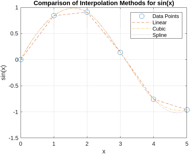
disp(yq);

Visualizing Interpolation Results using MATLAB interp1

% Define sample data points
x = [0 1 2 3 4 5];  % Known x-values
y = sin(x);         % Corresponding y-values using sin(x)

% Define query points
xq_vals = linspace(min(x), max(x), 100); 

% Perform interpolation using different methods
y_linear = interp1(x, y, xq_vals, 'linear');
y_cubic = interp1(x, y, xq_vals, 'cubic');
y_spline = interp1(x, y, xq_vals, 'spline');

% Plot original data points
figure;
plot(x, y, 'o', 'MarkerSize', 8, 'DisplayName', 'Data Points'); hold on;

% Plot interpolation results
plot(xq_vals, y_linear, '--', 'DisplayName', 'Linear');
plot(xq_vals, y_cubic, '-.', 'DisplayName', 'Cubic');
plot(xq_vals, y_spline, ':', 'DisplayName', 'Spline');

% Customize plot appearance
legend;
xlabel('x'); ylabel('sin(x)');
title('Comparison of Interpolation Methods for sin(x)');
grid on;

Handling Extrapolation in interp1 MATLAB

By default, interp1 returns NaN for query points outside the given range. To allow extrapolation, specify 'extrap'. This can be crucial when working with datasets requiring predictions beyond available points:

% Query points outside range
Xq_outside = [-1, 6];

% Linear extrapolation
Vq_extrap = interp1(X, V, Xq_outside, 'linear', 'extrap');

% Display result
disp(['Extrapolated values: ', num2str(Vq_extrap)]);

Real-World Example: Sensor Data Smoothing

Imagine you have sensor data sampled at irregular time intervals. You can use interp1 to create a smoother dataset with evenly spaced time steps.

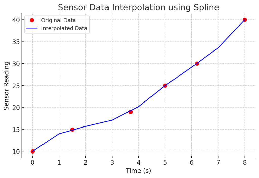
Advanced Features of interp1 in MATLAB

The MATLAB interp1 function provides a powerful tool for one-dimensional interpolation. While the basic usage is sufficient for simple scenarios, the advanced features allow users to tackle more complex problems, enhancing the capability of this function considerably. One notable feature is the ability to specify the ‘extrap’ option, which enables the extrapolation of data beyond the given data points. For instance, if the input data does not cover the desired range for interpolation, including the ‘extrap’ argument can help generate estimated values based on existing data trends, ensuring users can derive insights even in less populated data regions.

Handling missing data is another critical aspect of working with interpolation in MATLAB, and interp1 offers methods for managing NaN values effectively. When using this function, if the dataset contains any NaN entries, the resulting output will also be affected. To address this, users can choose to exclude NaNs before executing the interpolation or utilize the ‘linear’ interpolation method to fill in gaps with calculated values. This ensures that the final interpolated output remains robust, minimizing the impact of missing data points on the overall analysis.

Moreover, users can customize the output of the interp1 function to suit specific needs by employing various interpolation methods such as ‘spline’, ‘nearest’, and ‘cubic’. Each of these methods has its own characteristics and suitable applications with MATLAB, allowing users to select the most appropriate technique based on the behavior of their dataset. For example, spline interpolation provides smoother curves suitable for applications requiring high fidelity, while nearest interpolation can be beneficial in scenarios necessitating quick and straightforward estimates without complex calculations. These advanced features of MATLAB interp1 not only broaden its applicability but also provide flexibility in managing complex datasets, enabling users to extract meaningful information effectively.

Common Errors and Troubleshooting

The MATLAB interp1 function is a powerful tool for one-dimensional data interpolation, but users may occasionally face challenges that lead to errors or unexpected results. Understanding the common pitfalls associated with its use can help mitigate these issues. One frequent problem stems from incorrect data formats. When applying interp1, it’s crucial to ensure that the input vectors for the x and y data points are properly aligned. The x vector must be strictly increasing, and the corresponding y vector should maintain the same length. If the x values are not sorted correctly, MATLAB will return an error, prompting the user to verify their data arrangement.

Another common issue arises from mismatches in interpolation types. Users might inadvertently request an interpolation method that does not suit their data characteristics. For example, using the ‘nearest’ method on data that requires a smooth curve could yield misleading results. It is essential to select an appropriate interpolation type based on the nature of the data to achieve reliable and accurate output. Users can leverage the documentation provided by MATLAB to better understand the various interpolation methods available within the interp1 function.

To further troubleshoot issues encountered with the interp1 function, examining the size of the input arrays is also critical. If the x and y vectors differ in length, this discrepancy will prevent the function from executing correctly. MATLAB will highlight this issue, allowing users to redefine their data. Lastly, testing the function with a small sample set can aid in isolating the source of the problem, allowing for a clearer understanding of what adjustments might be needed. By paying attention to these common errors and implementing troubleshooting strategies, users can effectively use the MATLAB interp1 function to achieve their interpolation goals without unnecessary complications.

Practical Applications of MATLAB interp1 function

The interp1 function in MATLAB serves as a powerful tool for interpolation in diverse fields, including engineering, finance, and scientific research. This function is particularly beneficial for data analysis where gaps exist or where data points need to be estimated based on known values. In engineering, for example, it is frequently used in simulations where precise values of parameters are required. Engineers can utilize MATLAB interp1 to generate smooth curves from discrete data points, enabling better modeling of physical systems.

In the realm of financial analysis, the interp1 function allows analysts to estimate interest rates or stock prices when limited data points are available. By applying linear or spline interpolation, financial professionals can predict future trends, helping them make informed investment decisions. Case studies demonstrate its ability to fill gaps in historical data and thus enhance the accuracy of forecasting models.

Moreover, in scientific research, particularly in fields like meteorology and environmental science, interp1 is used to estimate atmospheric conditions based on recorded measurements. For instance, when reviewing temperature data collected at irregular intervals, researchers can apply MATLAB’s interpolation capabilities to derive a smoother dataset, aiding in climate modeling and analysis.

Another significant application can be found in the healthcare sector. Medical researchers often use interpolation to analyze patient data collected over varying time periods. Here, interp1 provides a method to standardize measurements, allowing for more effective comparisons and conclusions in clinical studies.

Overall, the use of MATLAB’s interp1 function across these various domains exemplifies its critical role in enabling accurate data interpretation and decision-making, significantly enhancing the quality of insights derived from numerical data sets.

Comparing MATLAB interp1 with Other Interpolation Functions

In MATLAB, the interp1 function is primarily utilized for one-dimensional interpolation. However, there are several other interpolation functions within MATLAB that serve distinct purposes, such as interp2 for two-dimensional data and griddata for irregularly spaced data. Understanding the differences between these functions helps users select the appropriate tool for their specific interpolation needs.

The interp2 function is designed for two-dimensional interpolation, making it suitable for applications where data is organized in a grid format, such as image processing or surface fitting. Users can perform bilinear and bicubic interpolation with interp2, effectively interpolating over both axes. In contrast, interp1 is limited to one-dimensional datasets, which means that for multi-dimensional scenarios, interp2 would be the recommended choice.

Another noteworthy function is griddata, which excels in interpolating data scattered on an irregular grid. Unlike interp1, which requires evenly spaced data points in one dimension, griddata allows for flexibility in data spacing, accommodating a broader range of applications. For instance, in geographical information systems (GIS), where data points can be erratic, griddata would often be favored for creating smooth, continuous surfaces from discrete points.

It is also essential to recognize that MATLAB provides different interpolation methods for each function, allowing users to choose based on their required accuracy and computational efficiency. Functions such as linear, spline, and nearest neighbor methods are available across these interpolation options, with selections varying in terms of smoothness and responsiveness to data fluctuations.

In summary, while interp1 is versatile for one-dimensional linear extrapolation and interpolation tasks, understanding when to implement interp2 or griddata can significantly advance the quality and applicability of data analysis across various dimensions.

Best Practices for Using interp1

The interp1 function in MATLAB is a powerful tool for one-dimensional interpolation; however, to achieve the best results, it is critical to adhere to certain best practices. First and foremost, conducting data validation prior to the interpolation process is essential. Ensure that the input data is free from NaN or infinite values, as these can lead to errors or unreliable output. Use functions such as isnan and isfinite to check for valid entries in your dataset. Furthermore, confirm that the vector of independent variables, often referred to as x, is sorted in ascending order, as unsorted data can lead to unpredictable behavior when applying interp1.

Secondly, selecting the appropriate interpolation method is vital for obtaining accurate results. The interp1 function provides several options: linear, nearest, spline, and pchip, among others. The choice of method depends on the nature of the data and the required smoothness of the output. For instance, linear interpolation is suitable for relatively linear datasets, while spline interpolation can yield smoother results for more complex datasets. Always consider testing different methods to determine which best meets your requirements, as this may significantly affect the interpolation accuracy.

Lastly, consider performance optimization when using the interp1 function, especially with large datasets. Using vectorized operations instead of loops can drastically enhance performance. Additionally, pre-allocating memory for the output array can prevent performance degradation when dealing with large arrays. Implementing these practices will not only improve the efficiency of the code but also increase the reliability of the interpolation results, allowing for more robust analytical work. By following these guidelines, you can adeptly utilize interp1 to its fullest potential in your MATLAB projects.

Other Functions in MATLAB

MATLAB Ode45 function – Practical Tutorials

Ode45 is a widely utilized numerical solver designed for the effective resolution of ordinary differential equations (ODEs). It is a part of MATLAB’s ODE suite and is specifically tailored to handle problems where the solution requires the calculation of derivatives at multiple points. The significance of Ode45 stems from its implementation of the Runge-Kutta method, which offers a robust approach to approximating solutions with high accuracy.

MATLAB Diff function – Beginners Tutorials

MATLAB diff function is an essential tool utilized in the realms of data analysis and programming. Primarily, it calculates the differences between adjacent elements in an array, offering valuable insights into trends and behaviors of data sets. Through a blend of theoretical understanding and hands-on practical examples, this guide aspires to empower readers to utilize MATLAB’s diff effectively, transforming raw data into actionable insights.

MATLAB conv2 Function

Convolution is a mathematical operation that combines two functions to produce a third function, expressing how the shape of one function is modified by the other. Convolution is calculated using MATLAB conv2 function. This operation is particularly crucial in various fields such as image processing, signal analysis, and systems engineering. This function is specifically designed for two-dimensional convolution, making it preferable for tasks that involve images or other matrix-based data

fft2 in MATLAB

The FFT2 function in MATLAB is crucial for performing Fourier transforms on matrices, allowing practitioners to study and manipulate two-dimensional frequency components effectively. The Fast Fourier Transform (FFT) is an algorithm that computes the discrete Fourier transform (DFT) and its inverse efficiently. The DFT converts a sequence of equally spaced samples of a function into a sequence of coefficients of sinusoidal components, revealing the frequency spectrum of the sampled signal.

fzero MATLAB Function

The fzero in MATLAB is a powerful tool designed for finding the roots of nonlinear equations. This function plays a crucial role in various fields, including engineering, data science, and mathematical modeling. By utilizing fzero MATLAB, users can efficiently identify points where a given function equals zero, which is essential for solving problems that involve polynomial equations, differential equations, and optimization tasks.