Euler Method in MATLAB

Euler Method with MATLAB

The Euler method, named after the Swiss mathematician Leonhard Euler, is a fundamental numerical technique widely used in mathematical analysis for solving ordinary differential equations (ODEs). In the realm of numerical analysis, many problems cannot be solved analytically, necessitating the use of numerical methods such as the Euler method to approximate solutions. Euler method can be solved in MATLAB and provides a straightforward approach to estimating the values of a function based on its initial conditions and the rate of change indicated by the differential equation.

This technique is particularly useful for first-order ODEs, which can often be expressed in the form of f'(y) = g(t, y). Here, the function f’ signifies the derivative of y with respect to t, and g(t, y) represents the relationship governing this change. The Euler method approximates the solution by employing the initial value of the dependent variable, combined with the slope derived from the function at that point, to calculate the subsequent value incrementally. This is done by iteratively applying the formula: y_{n+1} = y_n + h * f(t_n, y_n), where h is the step size determining how far to move in the t-direction with each iteration.

The Mathematical Theory Behind the Euler Method

The Euler method is a fundamental numerical technique for solving ordinary differential equations (ODEs), particularly initial value problems. It derives its roots from the Taylor series expansion, which provides a powerful means of approximating functions. The purpose of this method is to estimate the solution of a differential equation at discrete points by stepping forward in small increments from an initial condition.

To understand how the Euler method operates, consider a first-order ordinary differential equation expressed in the form (y’ = f(t, y)) with an initial condition (y(t_0) = y_0). The Taylor series expansion of (y) about (t_0) can be written as:

[y(t) = y(t_0) + (t – t_0) y'(t_0) + frac{(t – t_0)^2}{2} y”(t_0) + cdots]

For practical implementation, the Euler method truncates this series after the first-order term, leading to the approximation:

[y(t_0 + h) approx y(t_0) + h f(t_0, y_0)]

Here, (h) represents the step size, which is the distance between successive points in time. This simple formula illustrates the essence of the Euler method. It allows us to incrementally compute the solution by repeatedly applying the formula, progressing from the initial point (t_0) to any desired time (t_n). Thus, for (n) steps, the iterative formula becomes:

[y_{n+1} = y_n + h f(t_n, y_n)]

This process underscores the method’s explicit nature, which is easily implemented in various programming environments, such as MATLAB. In numerical analysis, the stability and accuracy of the Euler method are inherently linked to the size of (h); smaller values typically yield more precise results. Nonetheless, the choice of step size must balance computational efficiency and desired accuracy. The Euler method serves as a foundational approach in the numerical toolkit, setting the stage for more sophisticated methods that build upon its core principles.

Requirements for Implementing the Euler Method in MATLAB

To effectively implement the Euler method in MATLAB, a solid understanding of MATLAB basic syntax and programming environment is essential. Familiarity with basic programming concepts such as variables, loops, and functions will significantly enhance the coding experience. MATLAB operates using a matrix-based approach, which means that handling arrays and matrices efficiently is crucial when implementing numerical methods like Euler’s.

The first requirement is a basic grasp of MATLAB syntax. This includes understanding how to declare variables, perform basic operations, and utilize built-in functions. MATLAB is case-sensitive, so attention to detail is paramount. For instance, ‘variable’ and ‘Variable’ would be interpreted as two different entities. MATLAB treats most data types as matrices, so users should also be accustomed to matrix indexing and manipulation.

In addition to syntax, knowledge of essential MATLAB functions and operators is key. Functions such as ‘linspace’ for generating linearly spaced vectors, ‘plot’ for visualizing results, and ‘zeros’ for creating arrays are critical for implementing the Euler method. The Euler method itself involves iterative calculations that require looping constructs, especially the ‘for’ loop, which is used to execute a set sequence of commands repetitively.

Moreover, understanding the mathematical foundation of the Euler method will aid in its coding. The method computes the next value in a numerical solution based on the previous value and the function’s derivative at that point. Readers will benefit from reviewing differential equations and numerical analysis principles before embarking on their implementation. By ensuring familiarity with these prerequisites, developers can streamline their efforts to apply the Euler method in MATLAB effectively.

Learn MATLAB with Online Tutorials

Explore our MATLAB Online Tutorial, your ultimate guide to mastering MATLAB! Whether you’re a beginner or an advanced user, this guide covers everything from basic MATLAB concepts to advanced topics

Step-by-Step Implementation of the Euler Method in MATLAB

The Euler method is a fundamental numerical technique used to solve ordinary differential equations (ODEs). Implementing this method in MATLAB requires several systematic steps. Below, we provide a clear, step-by-step guide to coding the Euler method, including key examples that facilitate understanding.

First, start by defining the differential equation you aim to solve. For instance, consider the first-order ODE given by dy/dt = f(t, y). This equation needs to be rearranged to isolate dy on one side. In MATLAB, we can represent this function using an anonymous function:

f = @(t, y) -2 * y + 2 * cos(t);

Next, specify the initial conditions and the domain over which the solution will be computed. For our example, we assume an initial time t0, an initial value y0, and the ending time T. This could look like:

t0 = 0; y0 = 1
T = 10; h = 0.01
% Step sizeN = (T - t0) / h
% Number of iterations

After establishing the initial conditions, allocate arrays for t and y to store computed values:

t = zeros(1, N+1)
y = zeros(1, N+1)
t(1) = t0
y(1) = y0;

The core implementation of the Euler method involves a MATLAB for loop that iteratively updates the values of y based on the equation. This is carried out using the following code snippet:

for i = 1:Ny(i+1) = y(i) + h * f(t(i), y(i))
t(i+1) = t(i) + h
end

Finally, once the iterations are complete, you can visualize the results using MATLAB’s plotting functions. For example, to plot the computed solution against time, you could use:

plot(t, y)
xlabel('Time')
ylabel('Solution y(t)')
title('Euler Method Solution')
grid on;

This step-by-step implementation of the Euler method in MATLAB provides a basic but practical approach to numerically solving first-order ODEs, paving the way for further exploration and applications in various fields of study.

Let us define another problem and solve it using euler MALTAB methods

Setting Up the Problem

Before we implement Euler’s Method, let’s define the ODE we want to solve. Consider the differential equation:

Implementing Euler’s Method in MATLAB

Let’s break it down into logical steps. We start by defining the initial conditions, step size, and number of steps.

% Define the function dy/dx = f(x, y)
f = @(x, y) -2 * y;  % Example function

% Define initial conditions
x0 = 0;     % Initial x-value
y0 = 1;     % Initial y-value

% Define step size and number of steps
h = 0.1;    % Step size
N = 50;     % Number of steps (covers x=5)

We create arrays to store the computed values.

x = zeros(1, N+1);  % Preallocate for speed
y = zeros(1, N+1);

% Set initial values
x(1) = x0;
y(1) = y0;

We iterate on Euler’s formula using for loop in MATLAB.

for n = 1:N
    x(n+1) = x(n) + h;  % Increment x
    y(n+1) = y(n) + h * f(x(n), y(n));  % Compute y using Euler’s method
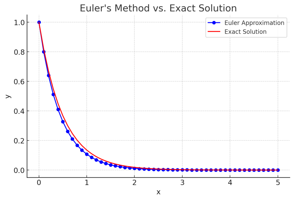
end

Visualization is key in understanding the accuracy of the method.

% Exact solution for comparison
y_exact = y0 * exp(-2 * x);

% Plot results
figure;
plot(x, y, 'bo-', 'LineWidth', 1.5);  % Euler's method
hold on;
plot(x, y_exact, 'r-', 'LineWidth', 1.5);  % Exact solution
hold off;

xlabel('x');
ylabel('y');
title("Euler's Method vs. Exact Solution");
legend('Euler Approximation', 'Exact Solution');
grid on;

Euler’s Method is a great starting point, but for better accuracy, consider:

• Improved Euler (Heun’s Method): Reduces error using an extra correction step.
• Runge-Kutta Methods (ode45 in MATLAB): More accurate for complex ODEs.
• MATLAB’s Built-in ODE Solvers: ode23, ode45, ode113, and ode15s handle stiff equations efficiently.

Example of using ode45 in MATLAB:

[x_ode, y_ode] = ode45(@(x,y) -2*y, [0 5], 1);
plot(x_ode, y_ode, 'g--', 'LineWidth', 1.5);
legend('Euler Approximation', 'Exact Solution', 'ode45 Solution');

Example Problem: Euler Method in Action

To illustrate the implementation of the Euler method in MATLAB, let us consider a simple first-order ordinary differential equation (ODE): dy/dt = -2y with an initial condition of y(0) = 1. This particular form of the equation describes exponential decay, which is a common scenario in various scientific fields such as physics and biology.

Firstly, we need to define the parameters for our simulation, including the time span and step size. For our example, we will simulate the system from t = 0 to t = 5 with a time step h = 0.1. To implement the Euler method, we will compute the next value of y using the formula: y_{n+1} = y_n + h * f(t_n, y_n), where f(t_n, y_n) is the right-hand side of the differential equation.

The following MATLAB code demonstrates how to implement the Euler method in this case:

t = 0:0.1:5
% Define the time vectory = zeros(size(t))
% Preallocate the solution arrayy(1) = 1
% Set initial conditionfor n = 1:length(t)-1y(n+1) = y(n) + (-2 * y(n)) * 0.1
% Apply the Euler formulaendplot(t, y)
% Plot the resultsxlabel('Time');ylabel('y(t)')
title('Euler Method Solution for dy/dt = -2y')
grid on;

After running this code in MATLAB, a plot of the solution will show the expected exponential decay of the function over the specified time span. The interpretation of the output reveals how well the Euler method approximates the solution of the differential equation. While it provides a reasonable estimate, it is essential to evaluate the accuracy of the results against more precise methods like the Runge-Kutta method, especially for more complex equations.

Common Errors and Troubleshooting Tips

When implementing the Euler method in MATLAB, users may encounter several common errors that can hinder the correct execution of their code. Identifying these pitfalls and employing effective troubleshooting strategies is essential for successful implementation of this numerical technique. One prevalent issue is the selection of an inappropriate step size. If the step size is too large, the solution may diverge significantly from the actual trajectory of the system being modeled. Conversely, a very small step size could lead to increased computation time without significant improvements in accuracy. It is advisable to test a range of step sizes to discover a balance that provides adequate precision while maintaining reasonable computational efficiency.

Another common error is incorrect implementation of the Euler formula. The basic computation step involves updating the dependent variable by adding the product of the derivative and the step size to the current value. Misplacing any components in this formula can lead to incorrect results. Care should be taken to double-check the implementation, ensuring that the order of operations is strictly followed. Additionally, ensure that the functions defined for the derivatives are implemented correctly and are properly defined within the MATLAB environment.

Moreover, users might encounter runtime errors related to variable dimensions. MATLAB is sensitive to matrix dimensions, and failing to initialize matrices or arrays correctly may result in dimension mismatch errors. To avoid this issue, preallocating memory for output matrices is a good practice. This ensures that MATLAB does not dynamically resize arrays during runtime, which can affect performance. Debugging tools such as breakpoints and the MATLAB debugger can also significantly assist in isolating the issues. By diligently applying these troubleshooting tips and understanding common errors associated with the Euler method in MATLAB, users can enhance the reliability and accuracy of their simulations.

Comparative Analysis: Euler Method vs. Other Numerical Methods

The Euler method is a foundational algorithm in numerical analysis, known for its simplicity in solving ordinary differential equations (ODEs). However, when comparing it to more advanced numerical methods, several key differences in terms of accuracy, computational efficiency, and ease of implementation become apparent. MATLAB diff function is another tool to solve differential equations.

One of the most commonly compared numerical methods is the Runge-Kutta method, particularly the fourth-order Runge-Kutta (RK4) variant. While the Euler method provides a straightforward approach to solving ODEs, it often falls short in terms of accuracy, especially when dealing with complex systems or higher-order equations. The Euler method approximates the solution using a straight line over an interval, which can lead to significant errors when the function behaves curvilinearly. In contrast, the RK4 method employs multiple intermediate steps to achieve a more accurate approximation of the trajectory, allowing it to maintain precision over larger intervals.

When considering computational efficiency, the Euler method has the advantage of low computational cost due to its simple calculations at each step. This makes it particularly appealing when speed is of the essence, such as in real-time simulations or scenarios with limited computing resources. However, this speed comes at a cost; to achieve comparable accuracy, the step size in the Euler method must often be reduced significantly, leading to a need for more iterations. Conversely, the Runge-Kutta methods tend to be more computationally intensive per step, but they can achieve higher accuracy with larger step sizes, resulting in fewer overall computations for many problems.

Finally, the ease of implementation of the Euler method cannot be overlooked. Its straightforward algorithm means that it is an excellent educational tool for those new to numerical methods. Nevertheless, as the need for precision increases, practitioners may find themselves gravitating toward methods like Runge-Kutta, which, while slightly more complex to implement, yield more reliable results for a broader range of applications. Understanding these distinctions is vital for selecting the appropriate method for any given problem.

Extending the Euler Method: Modifications and Variants

The Euler method, while straightforward and easy to implement in MATLAB, has limitations in terms of accuracy, particularly for stiff equations or when a high level of precision is required. Several modifications and variants of the Euler method have been developed to enhance its accuracy. Among these, the Improved Euler Method, also known as Heun’s method, is particularly notable. This variant involves taking an additional predictor step before the corrector step, which mitigates some of the errors inherent in the standard Euler approach.

In the Improved Euler Method, the process starts with an initial estimate using the standard Euler formula. Subsequently, a slope is computed using this prediction, which provides a more accurate representation of the behavior of the function within the interval. This averaged slope is then used to provide a refined approximation for the next step. Implementation of this method in Euler MATLAB is straightforward, enabling users to seamlessly integrate these modifications into their existing codebase. The Improved Euler Method can significantly reduce error propagation over long time intervals and is more stable for applications with rapidly changing dynamics.

Another category of modifications includes implicit methods, such as the Backward Euler method. Unlike the explicit approach of the standard Euler method, implicit methods require the solution of an algebraic equation at each time step, inherently improving stability for stiff systems. They are particularly useful in cases where the derivatives of the function exhibit significant changes, leading to potential numerical instability. Though the implicit methods can be more complex to implement within MATLAB due to the need for solving equations, their higher accuracy and stability make them invaluable for certain applications.

In summary, while the standard Euler method serves as an effective introductory technique for numerical solutions, modifications like the Improved Euler Method and implicit approaches offer enhanced accuracy and stability, making them preferable under specific conditions. These variants broaden the applicability of the Euler method in MATLAB, providing it with additional robustness suitable for a wider array of problems.

Conclusion and Further Reading

In this blog post, we explored the Euler method and its implementation in MATLAB, shedding light on its essential characteristics and applications in numerical analysis. The Euler method serves as a fundamental technique for solving ordinary differential equations (ODEs) by approximating solutions through iterative calculations. By using MATLAB, we have demonstrated how to apply this method effectively, highlighting its simplicity and accessibility for both beginners and experienced MATLAB users.

Throughout the discussion, we covered the theoretical foundation of the Euler method, illustrated the step-by-step implementation process within MATLAB, and provided MATLAB examples to solidify understanding. We also emphasized the importance of understanding the limitations associated with the Euler method, particularly regarding accuracy and stability, which can be crucial when dealing with more complex systems. Recognizing these limitations is vital for practitioners who must select the appropriate numerical method for their specific applications.

For readers interested in delving deeper into this topic, numerous resources and literature are available that cover the Euler method and other numerical methods in greater detail. Textbooks such as “Numerical Methods for Engineers” offer comprehensive insights into various numerical techniques, including the Euler method, while online courses on platforms like Coursera and edX provide practical exercises and additional context. Additionally, the MATLAB documentation serves as a valuable resource for learning more about its functions and capabilities in numerical analysis.

By enhancing your understanding of the Euler method in MATLAB and engaging with supplementary materials, you can broaden your knowledge base and become proficient in utilizing numerical methods for solving ODEs. As you continue to practice and implement these techniques, you will be better equipped to tackle more complex problems in your academic and professional endeavors.